搜索
Hi,
We are looking for users of Simulink who also work with the Vehicle Network toolbox to attend a usability session. This wil be a 2 hour session and will offer $100 compensation.
If you are interested, please answer the questions below and send them to: usabilityrecruiting@mathworks.com
In the past 2 years, how often have you worked with ARXML (AUTOSAR XML) files in vehicle network communication?
a. At least 3-5 days per week
b. Once or twice a week
c. A few times a month
d. Once a month or less
e. Never
-
3. Have you worked with automotive ethernet in the past?
a. Yes
b. No
-
4. Which of the following best describe your experience with Simulink? (select all that apply)
Study Screener Q4
a. I have used CAN/ CAN FD blocks (https://www.mathworks.com/help/vnt/can-simulink-communication.html)
b. I have used Simulink Buses
c. I have used Simulink Data Dictionaries
d. Other
-
Thank you!
Elaine
If you are interested in this session, just send an email with the answers to the following questions to usabilityrecruiting@mathworks.com
1. Which of the following best describes your experience with Design of Experiment (DOE)?
a. I regularly use DOE in my work and am comfortable designing experiments and analyzing results
b. I have used DOE in a few projects and understand its principles and applications
c. I have a basic understanding of DOE concepts but have limited practical experience
d. I have never used DOE but I’m interested in learning
-
2. Briefly describe one of your recent projects where you used/want to use DOE. What are the objectives and outcomes?
-
Thank you!
This website is not very attractive or easy to navigate. It is difficult to even find this section - if you start at the Mathworks website, there is no community tab:

You have to go to Help Center, which takes you to documentation, and then click on Community (redirecting you from https://www.mathworks.com/help to https://www.mathworks.com/matlabcentral)
Once you get there it's still a mess

If I have a question, it's not clear whether I should go to MATLAB Answers, Discussions, or Communities. It's not clear what the People page is for, or why it's split off from Community Advisors and Virtual Badges. "Cody" isn't very self-explanatory, and people will only stumble on it by accident, this seems like it should be integrated with contests. Don't get me started on the mess of a Blogs page. My browser knows that I speak English, so why am I being served Japanese language blogs?
I know that web design isn't the main priority of Mathworks, but the website has a very early-2010's look that increasingly feels dated. I hope there will be more consideration given to web UI/UX in the future.
I recently started learning MATLAB and Simulink, and I’m exploring the MathWorks website for study materials. Are there any free tutorials, examples, or beginner guides available directly from their official site? Also, are there special sections for students or personal users to access learning content without needing a full license?
In 2019, I wrote a MATLAB Central blog post called "The tool builder's gene (or how to get a job at MathWorks)." In it, I explained my personal theory of a characteristic of some engineers that is key for becoming successful software developers at MathWorks.
I just shared this essay on my personal blog, along with a couple of updates.
What is MATLAB Project?
39%
Never use it
28%
Only use existing from others' proj
3%
Use it occasionally
14%
Use it frequently
16%
88 个投票
clc; clear; close all;
% Initial guess for [x1, x2, x3] (adjust as needed)
x0 = [0.2,0.35,0.5];
% No linear constraints
A = []; b = [];
Aeq = []; beq = [];
% Lower and upper bounds (adjust based on the problem)
lb = [0,0,0];
ub = [pi/2,pi/2,pi/2];
% Optimization options
options = optimoptions('fmincon', 'Algorithm', 'sqp', 'Display', 'iter');
% Solve with fmincon
[x_opt, fval, exitflag] = fmincon(@objective, x0, A, b, Aeq, beq, lb, ub, @nonlinear_constraints, options);
% Display results
fprintf('Optimal Solution: x1 = %.4f, x2 = %.4f, x3 = %.4f\n', x_opt(1), x_opt(2), x_opt(3));
fprintf('Exit Flag: %d\n', exitflag);
%% Objective function (minimizing sum of squared errors)
function f = objective(x)
f = sum(x.^2); % Dummy function (since we only want to solve equations)
end
%% Nonlinear constraints (representing the trigonometric equations)
function [c, ceq] = nonlinear_constraints(x)
% Example nonlinear trigonometric equations:
ceq(1) = cos(x(1))+cos(x(2))+cos(x(3))-3*0.9; % First equation
ceq(2) = cos(5*x(1))+cos(5*x(2))+cos(5*x(3)); % Second equation
ceq(3) = cos(7*x(1))+cos(7*x(2))+cos(7*x(3)); % Third equation
c = [x(1)-x(2); x(2)-x(3)]; % No inequality constraints
end
Can anyone provide some matlab learning paths, I am a novice to MATLAB, I would appreciate it
I have written, tested, and prepared a function with four subsunctions on my computer for solving one of the problems in the list of Cody problems in MathWorks in three days. Today, when I wanted to upload or copy paste the codes of the function and its subfunctions to the specified place of the problem of Cody page, I do not see a place to upload it, and the ability to copy past the codes. The total of the entire codes and their documentations is about 600 lines, which means that I cannot and it is not worth it to retype all of them in the relevent Cody environment after spending a few days. I would appreciate your guidance on how to enter the prepared codes to the desired environment in Cody.
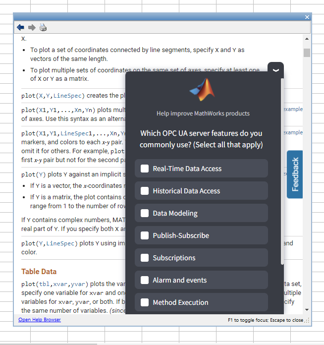
I'm getting this annoying survey (screenshot below) in the help windows of MATLAB R2024b this morning. It blocks the text I'm actually trying to read, when minimised it pops up again after a few minutes, and persists even after picking an option and completing the SurveyMonkey survey it links to. I don't even know what the OPC UA server so rest assured any of my answers to that survey aren't going to help MathWorks improve their product.
It is April 3, 2025 now. Where is the MATLAB 2025a?
There has been a lot of discussion here about the R2025a Prerelease that has really helped us get it ready for the prime time. Thank you for that!
A new update of the Prerelease has just dropped. So fresh it is still warm from the oven! In my latest blog post I discuss changes in the way MathWorks has been asking-for and processing feedback...and you have all been a part of that.
If you haven't tried the Prerelease in a while, I suggest you update and see how things are looking now.
If you have already submitted a bug report and it hasn't been fixed in this update, you don't need to submit another one. Everything is being tracked!
Have a play, discuss it here and thanks for again for being part of the process.
Hi! I'm Joseff and along with being a student in chemical engineering, one of my great passions is language-learning. I learnt something really cool recently about Catalan (a romance language closely related to Valencian that's spoken in Andorra, Catalonia, and parts of Spain) — and that is how speakers tell the time.
While most European languages stick to the standard minutes-past / minutes-to between hours, Catalan does something really quite special, with a focus on the quarters (quarts [ˈkwarts]). To see what I mean, take a look at this clock made by Penguin___Lover on Instructables :
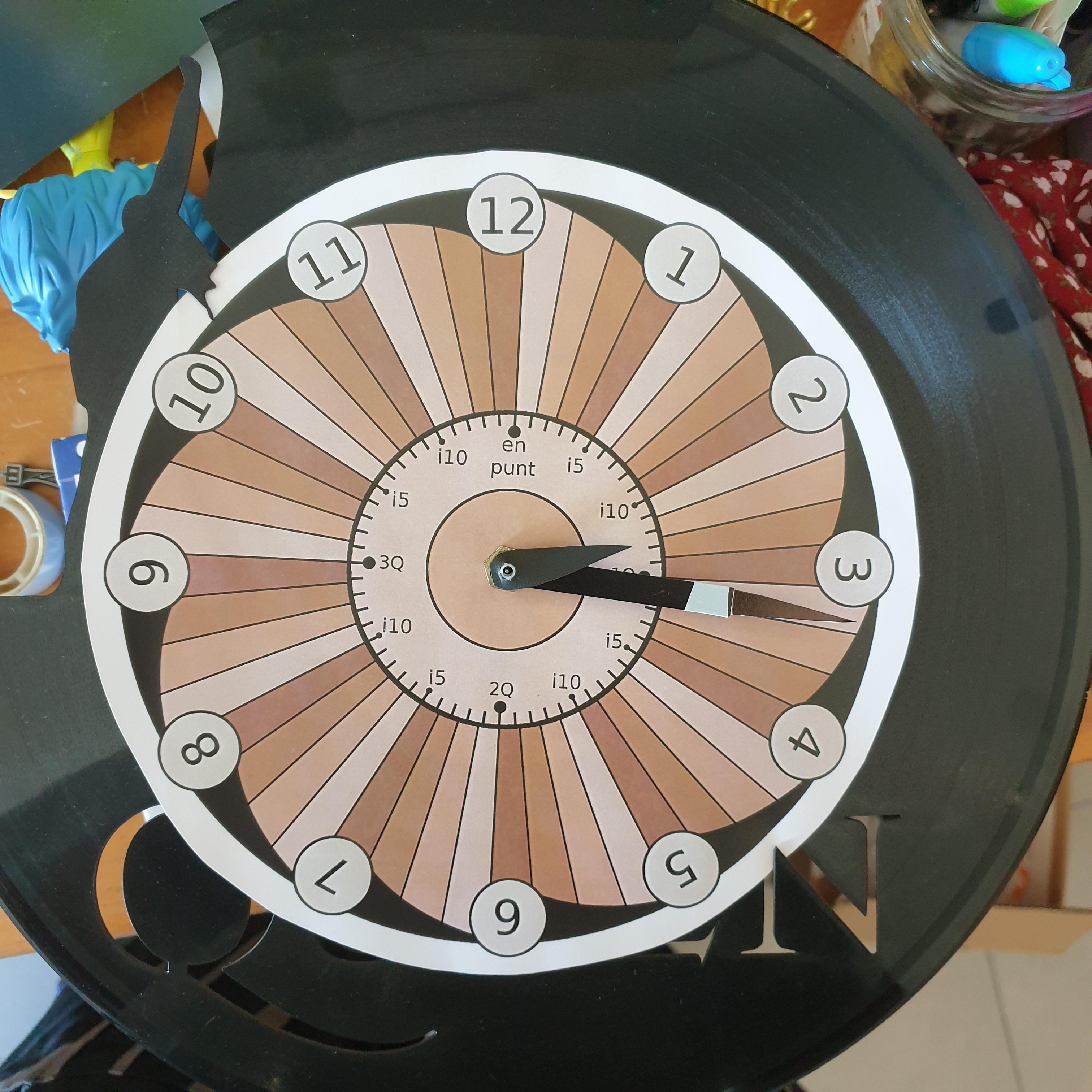
If you want to tell the time in Catalan, you should refer to the following hour (the one that's still to come), and how many minutes have passed or will pass for the closest quarter (sometimes half-quarter / mig quart [ˈmit͡ʃ kwart]) — clear as mud? It's definitely one of the more difficult things to wrap your head around as a learner. But fear not, with the power of MATLAB, we'll understand in no time!
To make a tool to tell the time in Catalan, the first thing we need to do is extract the current time into its individual hours, minutes and seconds*
function catalanTime = quinahora()
% Get the current time
[hours, minutes, seconds] = hms(datetime("now"));
% Adjust hours to 12-hour format
catalanHour = mod(hours-1, 12)+1;
nextHour = mod(hours, 12)+1;
Then to defining the numbers in catalan. It's worth noting that because the hours are feminine and the minutes are masculine, the words for 1 and 2 is different too (this is not too weird as languages go, in fact for my native Welsh there's a similar pattern between 2 and 4).
% Define the numbers in Catalan
catNumbers.masc = ["un", "dos", "tres", "quatre", "cinc"];
catNumbers.fem = ["una", "dues", "tres", "quatre",...
"cinc", "sis", "set", "vuit",...
"nou", "deu", "onze", "dotze"];
Okay, now it's starting to get serious! I mentioned before that this traditional time telling system is centred around the quarters — and that is true, but you'll also hear about the mig de quart (half of a quarter) * which is why we needed that seconds' precision from earlier!
% Define 07:30 intervals around the clock from 0 to 60
timeMarks = 0:15/2:60;
timeFraction = minutes + seconds / 60; % get the current position
[~, idx] = min(abs(timeFraction - timeMarks)); % extract the closest timeMark
mins = round(timeFraction - timeMarks(idx)); % round to the minute
After getting the fraction of the hour that we'll use later to tell the time, we can look into how many minutes it differs from that set time, using menys (less than) and i (on top of). There's also a bit of an AM/PM distinction, so you can use this function and know whether it's morning or night!
% Determine the minute string (diffString logic)
diffString = '';
if mins < 0
diffString = sprintf(' menys %s', catNumbers.masc(abs(mins)));
elseif mins > 0
diffString = sprintf(' i %s', catNumbers.masc(abs(mins)));
end
% Determine the part of the day (partofDay logic)
if hours < 12
partofDay = 'del matí'; % Morning (matí)
elseif hours < 18
partofDay = 'de la tarda'; % Afternoon (tarda)
elseif hours < 21
partofDay = 'del vespre'; % Evening (vespre)
else
partofDay = 'de la nit'; % Night (nit)
end
% Determine 'en punt' (o'clock exactly) based on minutes
enPunt = '';
if mins == 0
enPunt = ' en punt';
end
Now all that's left to do is define the main part of the string, which is which mig quart we are in. Since we extracted the index idx earlier as the closest timeMark, it's just a matter of indexing into this after the strings have been defined.
% Create the time labels
labels = {sprintf('són les %s%s%s %s', catNumbers.fem(catalanHour), diffString, enPunt, partofDay), ...
sprintf('és mig quart de %s%s %s', catNumbers.fem(nextHour), diffString, partofDay), ...
sprintf('és un quart de %s%s %s', catNumbers.fem(nextHour), diffString, partofDay), ...
sprintf('és un quart i mig de %s%s %s', catNumbers.fem(nextHour), diffString, partofDay), ...
sprintf('són dos quarts de %s%s %s', catNumbers.fem(nextHour), diffString, partofDay), ...
sprintf('són dos quarts i mig de %s%s %s', catNumbers.fem(nextHour), diffString, partofDay), ...
sprintf('són tres quarts de %s%s %s', catNumbers.fem(nextHour), diffString, partofDay), ...
sprintf('són tres quarts i mig de %s%s %s', catNumbers.fem(nextHour), diffString, partofDay), ...
sprintf('són les %s%s%s %s', catNumbers.fem(nextHour), diffString, enPunt, partofDay)};
catalanTime = labels{idx};
Then we need to do some clean up — the definite article les / la and the preposition de don't play nice with un and the initial vowel in onze, so there's a little replacement lookup here.
% List of old and new substrings for replacement
oldStrings = {'les un', 'són la una', 'de una', 'de onze'};
newStrings = {'la una', 'és la una', 'd''una', 'd''onze'};
% Apply replacements using a loop
for i = 1:length(oldStrings)
catalanTime = strrep(catalanTime, oldStrings{i}, newStrings{i});
end
end
quinahora()
So, can you work out what time it was when I made this post? 🤔
And how do you tell the time in your language?
Fins després!
📢 We want to hear from you! We're a team of graduate student researchers at the University of Michigan studying MATLAB Drive and other cloud-based systems for sharing coding files. Your feedback will help improve these tools. Take our quick survey here: https://forms.gle/DnHs4XNAwBZvmrAw6
No
50%
Yes, but I am not interested
8%
Yes, but it is too expensive
20%
Yes, I would like to know more
18%
Yes, I am cert. MATLAB Associate
2%
Yes, I am cert. MATLAB Professional
3%
4779 个投票
Over the last 5 years or so, the highest-traffic post on my MATLAB Central image processing blog was not actually about image processing; it was about changing the default line thickness in plots.
Now I have written about some other MATLAB plotting behavior that I have recently changed to suit my own preferences. See this new blog post.
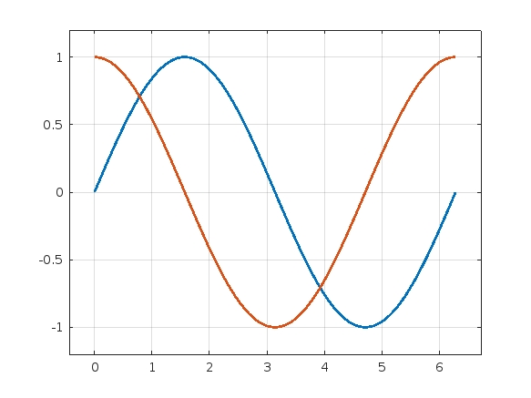
Here is a standard MATLAB plot:
x = 0:pi/100:2*pi;
y1 = sin(x);
y2 = cos(x);
plot(x,y1,x,y2)

I don't like some aspects of this plot, and so I have put the following code into my startup file.
set(groot,"DefaultLineLineWidth",2)
set(groot,"DefaultAxesXLimitMethod","padded")
set(groot,"DefaultAxesYLimitMethod","padded")
set(groot,"DefaultAxesZLimitMethod","padded")
set(groot,"DefaultAxesXGrid","on")
set(groot,"DefaultAxesYGrid","on")
set(groot,"DefaultAxesZGrid","on")
With those defaults changed, here is my preferred appearance:
plot(x,y1,x,y2)
To develop uifigure-based app, I wish MATLAB can provide something like uiquestdlg to replace questdlg without changing too much of the original code developed for figure-based app. Also, uiinputdlg <-> inputdlg and so on.
Learn the basic of quantum computing, how to simulate quantum circuits on MATLAB and how to run them on real quantum computers using Amazon Braket. There will also be a demonstration of machine learning using quantum computers!

Details at MATLAB-AMAZON Braket Hands-on Quantum Machine Learning Workshop - MATLAB & Simulink. This will be led by MathWorker Hossein Jooya.
I kicked off my own exploration of Quantum Computing in MATLAB a year or so ago and wrote it up on The MATLAB Blog: Quantum computing in MATLAB R2023b: On the desktop and in the cloud » The MATLAB Blog - MATLAB & Simulink. This made use of the MATLAB Support Package for Quantum Computing - File Exchange - MATLAB Central
Good day I am looking someone to help me on the matlab and simulink I am missing some explanations.For easy communication you can contact 0026876637042