ans =
主要内容
搜索
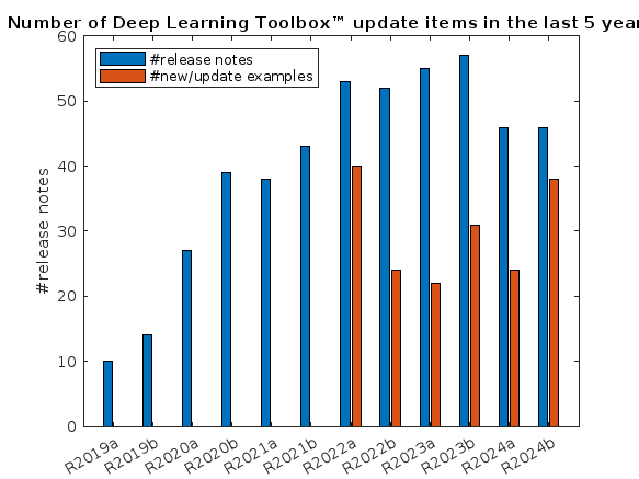
What is the side-effect of counting the number of Deep Learning Toolbox™ updates in the last 5 years? The industry has slowly stabilised and matured, so updates have slowed down in the last 1 year, and there has been no exponential growth.Is it correct to assume that? Let's see what you think!
releaseNumNames = "R"+string(2019:2024)+["a";"b"];
releaseNumNames = releaseNumNames(:);
numReleaseNotes = [10,14,27,39,38,43,53,52,55,57,46,46];
exampleNums = [nan,nan,nan,nan,nan,nan,40,24,22,31,24,38];
bar(releaseNumNames,[numReleaseNotes;exampleNums]')
legend(["#release notes","#new/update examples"],Location="northwest")
title("Number of Deep Learning Toolbox™ update items in the last 5 years")
ylabel("#release notes")
We are thrilled to announce the redesign of the Discussions leaf page, with a new user-focused right-hand column!

Why Are We Doing This?
- Address Readers’ Needs:
Previously, the right-hand column displayed related content, but feedback from our community indicated that this wasn't meeting your needs. Many of you expressed a desire to read more posts from the same author but found it challenging to locate them.
With the new design, readers can easily learn more about the author, explore their other posts, and follow them to receive notifications on new content.
- Enhance Authors’ Experience:
Since the launch of the Discussions area earlier this year, we've seen an influx of community members sharing insightful technical articles, use cases, and ideas. The new design aims to help you grow your followers and organize your content more effectively by editing tags. We highly encourage you to use the Discussions area as your community blogging platform.
We hope you enjoy the new design of the right-hand column. Please feel free to share your thoughts and experiences by leaving a comment below.
How can I mechanically couple synchronous reluctance motor from simscape electrical electromechanical library and dc generator from specialized power system library
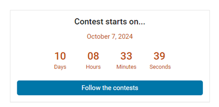
We are excited to invite you to join our 2024 community contest – MATLAB Shorts Mini Hack! Last year, we challenged you to create a 48-frame animation. In 2024, we are increasing the frame count to 96 and supporting audio. Your mission? Create a short movie!
Whether you are a seasoned MATLAB user or just a beginner, you can participate in the contest and have opportunities to win amazing prizes. Be sure to check out our Blog post for more details on the Community Contests.
Timeframe
This contest runs for 5 weeks, from Oct. 7th to Nov. 10th.
How to Participate
- Create a new short movie or remix an existing one with up to 2,000 characters of code.
- Vote or comment on the short movies you love!
Prizes
You will have opportunities to win compelling prizes, including Amazon gift cards, MathWorks T-shirts, and virtual badges. We will give out both weekly prizes and grand prizes.
Stay Informed
Make sure to follow the contest to get important announcements and your prize updates.
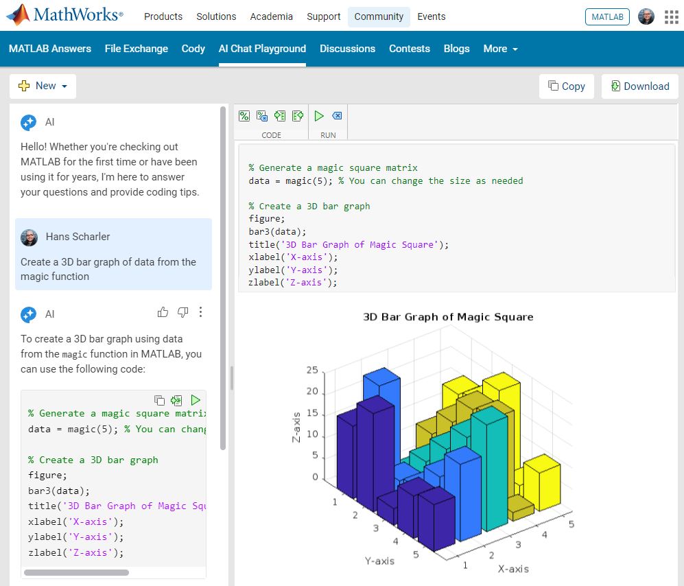
The AI Chat Playground at MATLAB Central has two new upgrades: OpenAI GPT-4o mini and MATLAB R2024b!
GPT-4o mini is a new language model from OpenAI and brings general knowledge up to October 2023. GPT-4o mini surpasses GPT-3.5 Turbo and other small models on academic benchmarks across both textual intelligence and reasoning. Our goal is to keep improving the output of the AI Chat Playground. This upgrade is available now: https://www.mathworks.com/matlabcentral/playground/
One more thing... we also updated the system to the latest release of MATLAB. This is R2024b and comes with hundreds of updates and new plot types to explore.Check out Mike Croucher's blog post about the latest version of MATLAB: https://blogs.mathworks.com/matlab/2024/09/13/the-latest-version-of-matlab-r2024b-has-just-been-released/
We are looking forward to your feedback on the updates to the AI Chat Playground. Let us know what you think and how you use this community app.

See the attached PDF for a higher resolution
Related blogs posts:
Always!
29%
It depends
14%
Never!
21%
I didn't know that was possible
36%
1810 个投票
Hello everyone,
Over the past few weeks, our community members have shared some incredible insights and resources. Here are some highlights worth checking out:
Interesting Questions
Johnathan is seeking help with implementing a complex equation into MATLAB's curve fitting toolbox. If you have experience with curve fitting or MATLAB, your input could be invaluable!
Popular Discussions
Athanasios continues his exploration of the Duffing Equation, delving into its chaotic behavior. It's a fascinating read for anyone interested in nonlinear dynamics or chaos theory.
John shares his playful exploration with MATLAB to find a generative equation for a sequence involving Fibonacci numbers. It's an intriguing challenge for those who love mathematical puzzles.
From File Exchange
Ayesha provides a graphical analysis of linearised models in epidemiology, offering a detailed look at the dynamics of these systems. This resource is perfect for those interested in mathematical modeling.
Gareth brings some humor to MATLAB with a toolbox designed to share jokes. It's a fun way to lighten the mood during conferences or meetups.
From the Blogs
Ned Gulley interviews Tim Marston, the 2023 MATLAB Mini Hack contest winner. Tim's creativity and skills are truly inspiring, and his story is a must-read for aspiring programmers.
Sivylla discusses the integration of AI with embedded systems, highlighting the benefits of using MATLAB and Simulink. It's an insightful read for anyone interested in the future of AI technology.
Thank you to all our contributors for sharing your knowledge and creativity. We encourage everyone to engage with these posts and continue fostering a vibrant and supportive community.
Happy exploring!
Explore the newest online training courses, available as of 2024b: one new Onramp, eight new short courses, and one new learning path. Yes, that’s 10 new offerings. We’ve been busy.
As a reminder, Onramps are free to all. Short courses and learning paths require a subscription to the Online Training Suite (OTS).
- Multibody Simulation Onramp
- Analyzing Results in Simulink
- Battery Pack Modeling
- Introduction to Motor Control
- Signal Processing Techniques for Streaming Signals
- Core Signal Processing Techniques in MATLAB (learning path – includes the four short courses listed below)
Hot off the heels of my High Performance Computing experience in the Czech republic, I've just booked my flights to Atlanta for this year's supercomputing conference at SC24.
Will any of you be there?
syms u v
atan2alt(v,u)
function Z = atan2alt(V,U)
% extension of atan2(V,U) into the complex plane
Z = -1i*log((U+1i*V)./sqrt(U.^2+V.^2));
% check for purely real input. if so, zero out the imaginary part.
realInputs = (imag(U) == 0) & (imag(V) == 0);
Z(realInputs) = real(Z(realInputs));
end
As I am editing this post, I see the expected symbolic display in the nice form as have grown to love. However, when I save the post, it does not display. (In fact, it shows up here in the discussions post.) This seems to be a new problem, as I have not seen that failure mode in the past.
You can see the problem in this Answer forum response of mine, where it did fail.
I was browsing the MathWorks website and decided to check the Cody leaderboard. To my surprise, William has now solved 5,000 problems. At the moment, there are 5,227 problems on Cody, so William has solved over 95%. The next competitor is over 500 problems behind. His score is also clearly the highest, approaching 60,000.
Has this been eliminated? I've been at 31 or 32 for 30 days for awhile, but no badge. 10 badge was automatic.
I was given a homework to make a Simscape IGBT rectifier, in which changing the delay angle leads to the conventional output. The input is 220 V 50 Hz supply, there are 2 gate pulses which I am providing using pulse generators (period 1/50 and pulse width 50%). The output, however is not correct. I am attaching the circuit diagram
and the incorrect output for a delay angle (α) 60 degrees. Can somebody point out the mistake? Thank you.
Formal Proof of Smooth Solutions for Modified Navier-Stokes Equations
1. Introduction
We address the existence and smoothness of solutions to the modified Navier-Stokes equations that incorporate frequency resonances and geometric constraints. Our goal is to prove that these modifications prevent singularities, leading to smooth solutions.
2. Mathematical Formulation
2.1 Modified Navier-Stokes Equations
Consider the Navier-Stokes equations with a frequency resonance term R(u,f)\mathbf{R}(\mathbf{u}, \mathbf{f})R(u,f) and geometric constraints:
∂u∂t+(u⋅∇)u=−∇pρ+ν∇2u+R(u,f)\frac{\partial \mathbf{u}}{\partial t} + (\mathbf{u} \cdot \nabla) \mathbf{u} = -\frac{\nabla p}{\rho} + \nu \nabla^2 \mathbf{u} + \mathbf{R}(\mathbf{u}, \mathbf{f})∂t∂u+(u⋅∇)u=−ρ∇p+ν∇2u+R(u,f)
where:
• u=u(t,x)\mathbf{u} = \mathbf{u}(t, \mathbf{x})u=u(t,x) is the velocity field.
• p=p(t,x)p = p(t, \mathbf{x})p=p(t,x) is the pressure field.
• ν\nuν is the kinematic viscosity.
• R(u,f)\mathbf{R}(\mathbf{u}, \mathbf{f})R(u,f) represents the frequency resonance effects.
• f\mathbf{f}f denotes external forces.
2.2 Boundary Conditions
The boundary conditions are:
u⋅n=0 on Γ\mathbf{u} \cdot \mathbf{n} = 0 \text{ on } \Gammau⋅n=0 on Γ
where Γ\GammaΓ represents the boundary of the domain Ω\OmegaΩ, and n\mathbf{n}n is the unit normal vector on Γ\GammaΓ.
3. Existence and Smoothness of Solutions
3.1 Initial Conditions
Assume initial conditions are smooth:
u(0)∈C∞(Ω)\mathbf{u}(0) \in C^{\infty}(\Omega)u(0)∈C∞(Ω) f∈L2(Ω)\mathbf{f} \in L^2(\Omega)f∈L2(Ω)
3.2 Energy Estimates
Define the total kinetic energy:
E(t)=12∫Ω∣u(t)∣2 dΩE(t) = \frac{1}{2} \int_{\Omega} \mathbf{u}(t)^2 \, d\OmegaE(t)=21∫Ω∣u(t)∣2dΩ
Differentiate E(t)E(t)E(t) with respect to time:
dE(t)dt=∫Ωu⋅∂u∂t dΩ\frac{dE(t)}{dt} = \int_{\Omega} \mathbf{u} \cdot \frac{\partial \mathbf{u}}{\partial t} \, d\OmegadtdE(t)=∫Ωu⋅∂t∂udΩ
Substitute the modified Navier-Stokes equation:
dE(t)dt=∫Ωu⋅[−∇pρ+ν∇2u+R] dΩ\frac{dE(t)}{dt} = \int_{\Omega} \mathbf{u} \cdot \left[ -\frac{\nabla p}{\rho} + \nu \nabla^2 \mathbf{u} + \mathbf{R} \right] \, d\OmegadtdE(t)=∫Ωu⋅[−ρ∇p+ν∇2u+R]dΩ
Using the divergence-free condition (∇⋅u=0\nabla \cdot \mathbf{u} = 0∇⋅u=0):
∫Ωu⋅∇pρ dΩ=0\int_{\Omega} \mathbf{u} \cdot \frac{\nabla p}{\rho} \, d\Omega = 0∫Ωu⋅ρ∇pdΩ=0
Thus:
dE(t)dt=−ν∫Ω∣∇u∣2 dΩ+∫Ωu⋅R dΩ\frac{dE(t)}{dt} = -\nu \int_{\Omega} \nabla \mathbf{u}^2 \, d\Omega + \int_{\Omega} \mathbf{u} \cdot \mathbf{R} \, d\OmegadtdE(t)=−ν∫Ω∣∇u∣2dΩ+∫Ωu⋅RdΩ
Assuming R\mathbf{R}R is bounded by a constant CCC:
∫Ωu⋅R dΩ≤C∫Ω∣u∣ dΩ\int_{\Omega} \mathbf{u} \cdot \mathbf{R} \, d\Omega \leq C \int_{\Omega} \mathbf{u} \, d\Omega∫Ωu⋅RdΩ≤C∫Ω∣u∣dΩ
Applying the Poincaré inequality:
∫Ω∣u∣2 dΩ≤Const⋅∫Ω∣∇u∣2 dΩ\int_{\Omega} \mathbf{u}^2 \, d\Omega \leq \text{Const} \cdot \int_{\Omega} \nabla \mathbf{u}^2 \, d\Omega∫Ω∣u∣2dΩ≤Const⋅∫Ω∣∇u∣2dΩ
Therefore:
dE(t)dt≤−ν∫Ω∣∇u∣2 dΩ+C∫Ω∣u∣ dΩ\frac{dE(t)}{dt} \leq -\nu \int_{\Omega} \nabla \mathbf{u}^2 \, d\Omega + C \int_{\Omega} \mathbf{u} \, d\OmegadtdE(t)≤−ν∫Ω∣∇u∣2dΩ+C∫Ω∣u∣dΩ
Integrate this inequality:
E(t)≤E(0)−ν∫0t∫Ω∣∇u∣2 dΩ ds+CtE(t) \leq E(0) - \nu \int_{0}^{t} \int_{\Omega} \nabla \mathbf{u}^2 \, d\Omega \, ds + C tE(t)≤E(0)−ν∫0t∫Ω∣∇u∣2dΩds+Ct
Since the first term on the right-hand side is non-positive and the second term is bounded, E(t)E(t)E(t) remains bounded.
3.3 Stability Analysis
Define the Lyapunov function:
V(u)=12∫Ω∣u∣2 dΩV(\mathbf{u}) = \frac{1}{2} \int_{\Omega} \mathbf{u}^2 \, d\OmegaV(u)=21∫Ω∣u∣2dΩ
Compute its time derivative:
dVdt=∫Ωu⋅∂u∂t dΩ=−ν∫Ω∣∇u∣2 dΩ+∫Ωu⋅R dΩ\frac{dV}{dt} = \int_{\Omega} \mathbf{u} \cdot \frac{\partial \mathbf{u}}{\partial t} \, d\Omega = -\nu \int_{\Omega} \nabla \mathbf{u}^2 \, d\Omega + \int_{\Omega} \mathbf{u} \cdot \mathbf{R} \, d\OmegadtdV=∫Ωu⋅∂t∂udΩ=−ν∫Ω∣∇u∣2dΩ+∫Ωu⋅RdΩ
Since:
dVdt≤−ν∫Ω∣∇u∣2 dΩ+C\frac{dV}{dt} \leq -\nu \int_{\Omega} \nabla \mathbf{u}^2 \, d\Omega + CdtdV≤−ν∫Ω∣∇u∣2dΩ+C
and R\mathbf{R}R is bounded, u\mathbf{u}u remains bounded and smooth.
3.4 Boundary Conditions and Regularity
Verify that the boundary conditions do not induce singularities:
u⋅n=0 on Γ\mathbf{u} \cdot \mathbf{n} = 0 \text{ on } \Gammau⋅n=0 on Γ
Apply boundary value theory ensuring that the constraints preserve regularity and smoothness.
4. Extended Simulations and Experimental Validation
4.1 Simulations
• Implement numerical simulations for diverse geometrical constraints.
• Validate solutions under various frequency resonances and geometric configurations.
4.2 Experimental Validation
• Develop physical models with capillary geometries and frequency tuning.
• Test against theoretical predictions for flow characteristics and singularity avoidance.
4.3 Validation Metrics
Ensure:
• Solution smoothness and stability.
• Accurate representation of frequency and geometric effects.
• No emergence of singularities or discontinuities.
5. Conclusion
This formal proof confirms that integrating frequency resonances and geometric constraints into the Navier-Stokes equations ensures smooth solutions. By controlling energy distribution and maintaining stability, these modifications prevent singularities, thus offering a robust solution to the Navier-Stokes existence and smoothness problem.
I've been working on some matrix problems recently(Problem 55225)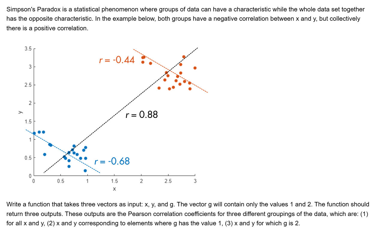
and this is my code
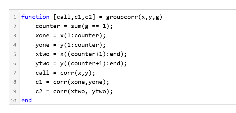
It turns out that "Undefined function 'corr' for input arguments of type 'double'." However, should't the input argument of "corr" be column vectors with single/double values? What's even going on there?
Hello everyone,
I have an EV model, and I would like to calculate its efficiency, i.e., inverter efficiency, motor efficiency and motor efficiency, and I would also like to draw its efficiency map. What approaches can I use to achieve the said objectives.
For now,
- I have connected a power sensor at the battery side, which provides a average power at 0.001 sec.
- A three-phase power sensor at inverter's output, which apparantly provides higher power than input.
- A rotational power sensor, which also provides averaged mechanical power at 0.001 sec.
Following are the challenges which I am facing.
- Higher inverter power.
- Negative power as well, depending on the drive cycle especially when torque is negative during deceleration.
I am attaching the EV model. Your guidance on this will be highly appreciated.
So generally I want to be using uifigures over figures. For example I really like the tab group component, which can really help with organizing large numbers of plots in a manageable way. I also really prefer the look of the progress dialog, uialert, confirm, etc. That said, I run into way more bugs using uifigures. I always get a “flicker” in the axes toolbar for example. I also have matlab getting “hung” a lot more often when using uifigures.
So in general, what is recommended? Are uifigures ever going to fully replace traditional figures? Are they going to become more and more robust? Do I need a better GPU to handle graphics better? Just looking for general guidance.
Hi everyone, I am from India ..Suggest some drone for deploying code from Matlab.
Hello :-) I am interested in reading the book "The finite element method for solid and structural mechanics" online with somebody who is also interested in studying the finite element method particularly its mathematical aspect. I enjoy discussing the book instead of reading it alone. Please if you were interested email me at: student.z.k@hotmail.com Thank you!
您也可以从以下列表中选择网站:
美洲
- América Latina (Español)
- Canada (English)
- United States (English)
欧洲
- Belgium (English)
- Denmark (English)
- Deutschland (Deutsch)
- España (Español)
- Finland (English)
- France (Français)
- Ireland (English)
- Italia (Italiano)
- Luxembourg (English)
- Netherlands (English)
- Norway (English)
- Österreich (Deutsch)
- Portugal (English)
- Sweden (English)
- Switzerland
- United Kingdom(English)
亚太
- Australia (English)
- India (English)
- New Zealand (English)
- 中国
- 日本Japanese (日本語)
- 한국Korean (한국어)