搜索
In the sequence of previous suggestion in Meta Cody comment for the 'My Problems' page, I also suggest to add a red alert for new comments in 'My Groups' page.
Thank you in advance.
(Requested for newer MATLAB releases (e.g. R2026B), MATLAB Parallel Processing toolbox.)
Lower precision array types have been gaining more popularity over the years for deep learning. The current lowest precision built-in array type offered by MATLAB are 8-bit precision arrays, e.g. int8 and uint8. A good thing is that these 8-bit array types do have gpuArray support, meaning that one is able to design GPU MEX codes that take in these 8-bit arrays and reinterpret them bit-wise as other 8-bit array types, e.g. FP8, which is especially common array type used in modern day deep learning applications. I myself have used this to develop forward pass operations with 8-bit precision that are around twice as fast as 16-bit operations and with output arrays that still agree well with 16-bit outputs (measured with high cosine similarity). So the 8-bit support that MATLAB offers is already quite sufficient.
Recently, 4-bit precision array types have been shown also capable of being very useful in deep learning. These array types can be processed with Tensor Cores of more modern GPUs, such as NVIDIA's Blackwell architecture. However, MATLAB does not yet have a built-in 4-bit precision array type.
Just like MATLAB has int8 and uint8, both also with gpuArray support, it would also be nice to have MATLAB have int4 and uint4, also with gpuArray support.
I can't believe someone put time into this ;-)

Our exportgraphics and copygraphics functions now offer direct and intuitive control over the size, padding, and aspect ratio of your exported figures.
- Specify Output Size: Use the new Width, Height, and Units name-value pairs
- Control Padding: Easily adjust the space around your axes using the Padding argument, or set it to to match the onscreen appearance.
- Preserve Aspect Ratio: Use PreserveAspectRatio='on' to maintain the original plot proportions when specifying a fixed size.
- SVG Export: The exportgraphics function now supports exporting to the SVG file format.
Check out the full article on the Graphics and App Building blog for examples and details: Advanced Control of Size and Layout of Exported Graphics
No, staying home (or where I'm now)
25%
Yes, 1 night
0%
Yes, 2 nights
12.5%
Yes, 3 nights
12.5%
Yes, 4-7 nights
25%
Yes, 8 nights or more
25%
8 个投票
I believe that it is very useful and important to know when we have new comments of our own problems. Although I had chosen to receive notifications about my own problems, I only receive them when I am mentioned by @.
Is it possible to add a 'New comment' alert in front of each problem on the 'My Problems' page?

The formula comes from @yuruyurau. (https://x.com/yuruyurau)
digital life 1

figure('Position',[300,50,900,900], 'Color','k');
axes(gcf, 'NextPlot','add', 'Position',[0,0,1,1], 'Color','k');
axis([0, 400, 0, 400])
SHdl = scatter([], [], 2, 'filled','o','w', 'MarkerEdgeColor','none', 'MarkerFaceAlpha',.4);
t = 0;
i = 0:2e4;
x = mod(i, 100);
y = floor(i./100);
k = x./4 - 12.5;
e = y./9 + 5;
o = vecnorm([k; e])./9;
while true
t = t + pi/90;
q = x + 99 + tan(1./k) + o.*k.*(cos(e.*9)./4 + cos(y./2)).*sin(o.*4 - t);
c = o.*e./30 - t./8;
SHdl.XData = (q.*0.7.*sin(c)) + 9.*cos(y./19 + t) + 200;
SHdl.YData = 200 + (q./2.*cos(c));
drawnow
end
digital life 2

figure('Position',[300,50,900,900], 'Color','k');
axes(gcf, 'NextPlot','add', 'Position',[0,0,1,1], 'Color','k');
axis([0, 400, 0, 400])
SHdl = scatter([], [], 2, 'filled','o','w', 'MarkerEdgeColor','none', 'MarkerFaceAlpha',.4);
t = 0;
i = 0:1e4;
x = i;
y = i./235;
e = y./8 - 13;
while true
t = t + pi/240;
k = (4 + sin(y.*2 - t).*3).*cos(x./29);
d = vecnorm([k; e]);
q = 3.*sin(k.*2) + 0.3./k + sin(y./25).*k.*(9 + 4.*sin(e.*9 - d.*3 + t.*2));
SHdl.XData = q + 30.*cos(d - t) + 200;
SHdl.YData = 620 - q.*sin(d - t) - d.*39;
drawnow
end
digital life 3

figure('Position',[300,50,900,900], 'Color','k');
axes(gcf, 'NextPlot','add', 'Position',[0,0,1,1], 'Color','k');
axis([0, 400, 0, 400])
SHdl = scatter([], [], 1, 'filled','o','w', 'MarkerEdgeColor','none', 'MarkerFaceAlpha',.4);
t = 0;
i = 0:1e4;
x = mod(i, 200);
y = i./43;
k = 5.*cos(x./14).*cos(y./30);
e = y./8 - 13;
d = (k.^2 + e.^2)./59 + 4;
a = atan2(k, e);
while true
t = t + pi/20;
q = 60 - 3.*sin(a.*e) + k.*(3 + 4./d.*sin(d.^2 - t.*2));
c = d./2 + e./99 - t./18;
SHdl.XData = q.*sin(c) + 200;
SHdl.YData = (q + d.*9).*cos(c) + 200;
drawnow; pause(1e-2)
end
digital life 4

figure('Position',[300,50,900,900], 'Color','k');
axes(gcf, 'NextPlot','add', 'Position',[0,0,1,1], 'Color','k');
axis([0, 400, 0, 400])
SHdl = scatter([], [], 1, 'filled','o','w', 'MarkerEdgeColor','none', 'MarkerFaceAlpha',.4);
t = 0;
i = 0:4e4;
x = mod(i, 200);
y = i./200;
k = x./8 - 12.5;
e = y./8 - 12.5;
o = (k.^2 + e.^2)./169;
d = .5 + 5.*cos(o);
while true
t = t + pi/120;
SHdl.XData = x + d.*k.*sin(d.*2 + o + t) + e.*cos(e + t) + 100;
SHdl.YData = y./4 - o.*135 + d.*6.*cos(d.*3 + o.*9 + t) + 275;
SHdl.CData = ((d.*sin(k).*sin(t.*4 + e)).^2).'.*[1,1,1];
drawnow;
end
digital life 5

figure('Position',[300,50,900,900], 'Color','k');
axes(gcf, 'NextPlot','add', 'Position',[0,0,1,1], 'Color','k');
axis([0, 400, 0, 400])
SHdl = scatter([], [], 1, 'filled','o','w',...
'MarkerEdgeColor','none', 'MarkerFaceAlpha',.4);
t = 0;
i = 0:1e4;
x = mod(i, 200);
y = i./55;
k = 9.*cos(x./8);
e = y./8 - 12.5;
while true
t = t + pi/120;
d = (k.^2 + e.^2)./99 + sin(t)./6 + .5;
q = 99 - e.*sin(atan2(k, e).*7)./d + k.*(3 + cos(d.^2 - t).*2);
c = d./2 + e./69 - t./16;
SHdl.XData = q.*sin(c) + 200;
SHdl.YData = (q + 19.*d).*cos(c) + 200;
drawnow;
end
digital life 6

clc; clear
figure('Position',[300,50,900,900], 'Color','k');
axes(gcf, 'NextPlot','add', 'Position',[0,0,1,1], 'Color','k');
axis([0, 400, 0, 400])
SHdl = scatter([], [], 2, 'filled','o','w', 'MarkerEdgeColor','none', 'MarkerFaceAlpha',.4);
t = 0;
i = 1:1e4;
y = i./790;
k = y; idx = y < 5;
k(idx) = 6 + sin(bitxor(floor(y(idx)), 1)).*6;
k(~idx) = 4 + cos(y(~idx));
while true
t = t + pi/90;
d = sqrt((k.*cos(i + t./4)).^2 + (y/3-13).^2);
q = y.*k.*cos(i + t./4)./5.*(2 + sin(d.*2 + y - t.*4));
c = d./3 - t./2 + mod(i, 2);
SHdl.XData = q + 90.*cos(c) + 200;
SHdl.YData = 400 - (q.*sin(c) + d.*29 - 170);
drawnow; pause(1e-2)
end
digital life 7

clc; clear
figure('Position',[300,50,900,900], 'Color','k');
axes(gcf, 'NextPlot','add', 'Position',[0,0,1,1], 'Color','k');
axis([0, 400, 0, 400])
SHdl = scatter([], [], 2, 'filled','o','w', 'MarkerEdgeColor','none', 'MarkerFaceAlpha',.4);
t = 0;
i = 1:1e4;
y = i./345;
x = y; idx = y < 11;
x(idx) = 6 + sin(bitxor(floor(x(idx)), 8))*6;
x(~idx) = x(~idx)./5 + cos(x(~idx)./2);
e = y./7 - 13;
while true
t = t + pi/120;
k = x.*cos(i - t./4);
d = sqrt(k.^2 + e.^2) + sin(e./4 + t)./2;
q = y.*k./d.*(3 + sin(d.*2 + y./2 - t.*4));
c = d./2 + 1 - t./2;
SHdl.XData = q + 60.*cos(c) + 200;
SHdl.YData = 400 - (q.*sin(c) + d.*29 - 170);
drawnow; pause(5e-3)
end
digital life 8

clc; clear
figure('Position',[300,50,900,900], 'Color','k');
axes(gcf, 'NextPlot','add', 'Position',[0,0,1,1], 'Color','k');
axis([0, 400, 0, 400])
SHdl{6} = [];
for j = 1:6
SHdl{j} = scatter([], [], 2, 'filled','o','w', 'MarkerEdgeColor','none', 'MarkerFaceAlpha',.3);
end
t = 0;
i = 1:2e4;
k = mod(i, 25) - 12;
e = i./800; m = 200;
theta = pi/3;
R = [cos(theta) -sin(theta); sin(theta) cos(theta)];
while true
t = t + pi/240;
d = 7.*cos(sqrt(k.^2 + e.^2)./3 + t./2);
XY = [k.*4 + d.*k.*sin(d + e./9 + t);
e.*2 - d.*9 - d.*9.*cos(d + t)];
for j = 1:6
XY = R*XY;
SHdl{j}.XData = XY(1,:) + m;
SHdl{j}.YData = XY(2,:) + m;
end
drawnow;
end
digital life 9

clc; clear
figure('Position',[300,50,900,900], 'Color','k');
axes(gcf, 'NextPlot','add', 'Position',[0,0,1,1], 'Color','k');
axis([0, 400, 0, 400])
SHdl{14} = [];
for j = 1:14
SHdl{j} = scatter([], [], 2, 'filled','o','w', 'MarkerEdgeColor','none', 'MarkerFaceAlpha',.1);
end
t = 0;
i = 1:2e4;
k = mod(i, 50) - 25;
e = i./1100; m = 200;
theta = pi/7;
R = [cos(theta) -sin(theta); sin(theta) cos(theta)];
while true
t = t + pi/240;
d = 5.*cos(sqrt(k.^2 + e.^2) - t + mod(i, 2));
XY = [k + k.*d./6.*sin(d + e./3 + t);
90 + e.*d - e./d.*2.*cos(d + t)];
for j = 1:14
XY = R*XY;
SHdl{j}.XData = XY(1,:) + m;
SHdl{j}.YData = XY(2,:) + m;
end
drawnow;
end
Hello everyone,
My name is heavnely, studying Aerospace Enginerring in IIT Kharagpur. I'm trying to meet people that can help to explore about things in control systems, drones, UAV, Reseearch. I have started wrting papers an year ago and hopefully it is going fine. I hope someone would reply to reply to this messege.
Thank you so much for anyone who read my messege.
In https://www.mathworks.com/matlabcentral/answers/38165-how-to-remove-decimal#comment_3345149 @Luisa asks,
@Cody Team, how can I vote or give a like in great comments?
It seems that there are not such options.
Developing an application in MATLAB often feels like a natural choice: it offers a unified environment, powerful visualization tools, accessible syntax, and a robust technical ecosystem. But when the goal is to build a compilable, distributable app, the path becomes unexpectedly difficult if your workflow depends on symbolic functions like sym, zeta, or lambertw.
This isn’t a minor technical inconvenience—it’s a structural contradiction. MATLAB encourages the creation of graphical interfaces, input validation, and dynamic visualization. It even provides an Application Compiler to package your code. But the moment you invoke sym, the compiler fails. No clear warning. No workaround. Just: you cannot compile. The same applies to zeta and lambertw, which rely on the symbolic toolbox.
So we’re left asking: how can a platform designed for scientific and technical applications block compilation of functions that are central to those very disciplines?
What Are the Alternatives?
- Rewrite everything numerically, avoiding symbolic logic—often impractical for advanced mathematical workflows.
- Use partial workarounds like matlabFunction, which may work but rarely preserve the original logic or flexibility.
- Switch platforms (e.g., Python with SymPy, Julia), which means rebuilding the architecture and leaving behind MATLAB’s ecosystem.
So, Is MATLAB Still Worth It?
That’s the real question. MATLAB remains a powerful tool for prototyping, teaching, analysis, and visualization. But when it comes to building compilable apps that rely on symbolic computation, the platform imposes limits that contradict its promise.
Is it worth investing time in a MATLAB app if you can’t compile it due to essential mathematical functions? Should MathWorks address this contradiction? Or is it time to rethink our tools?
I’d love to hear your thoughts. Is MATLAB still worth it for serious application development?
Pure Matlab
82%
Simulink
18%
11 个投票
If you have solved a Cody problem before, you have likely seen the Scratch Pad text field below the Solution text field. It provides a quick way to get feedback on your solution before submitting it. Since submitting a solution takes you to a new page, any time a wrong solution is submitted, you have to navigate back to the problem page to try it again.
Instead, I use the Scratch Pad to test my solution repeatedly before submitting. That way, I get to a working solution faster without having to potentially go back and forth many times between the problem page and the wrong-solution page.
Here is my approach:
- Write a tentative solution.
- Copy a test case from the test suite into the Scratch Pad.
- Click the Run Function button—this is immediately below the Scratch Pad and above the Output panel and Submit buttons.
- If the solution does not work, modify the solution code, sometimes putting in disp() lines and/or removing semicolons to trace what the code is doing. Repeat until the solution passes.
- If the solution does work, repeat steps 2 through 4.
- Once there are no more test cases to copy and paste, clean up the code, if necessary (delete disp lines, reinstate all semicolons to suppress output). Click the Run Function button once more, just to make sure I did not break the solution while cleaning it up. Then, click the Submit button.
For problems with large test suites, you may find it useful to copy and paste in multiple test cases per iteration.
Hopefully you find this useful.
Title: Looking for Internship Guidance as a Beginner MATLAB/Simulink Learner
Hello everyone,
I’m a Computer Science undergraduate currently building a strong foundation in MATLAB and Simulink. I’m still at a beginner level, but I’m actively learning every day and can work confidently once I understand the concepts. Right now I’m focusing on MATLAB modeling, physics simulation, and basic control systems so that I can contribute effectively to my current project.
I’m part of an Autonomous Underwater Vehicle (AUV) team preparing for the Singapore AUV Challenge (SAUVC). My role is in physics simulation, controls, and navigation, and MATLAB/Simulink plays a major role in that pipeline. I enjoy physics and mathematics deeply, which makes learning modeling and simulation very exciting for me.
On the coding side, I practice competitive programming regularly—
• Codeforces rating: ~1200
• LeetCode rating: ~1500
So I'm comfortable with logic-building and problem solving. What I’m looking for:
I want to know how a beginner like me can start applying for internships related to MATLAB, Simulink, modeling, simulation, or any engineering team where MATLAB is widely used (including companies outside MathWorks).
I would really appreciate advice from the community on:
- What skills should I strengthen first?
- Which MATLAB/Simulink toolboxes are most important for beginners aiming toward simulation/control roles?
- What small projects or portfolio examples should I build to improve my profile?
- What is the best roadmap to eventually become a good candidate for internships in this area?
Any guidance, resources, or suggestions would be extremely helpful for me.
Thank you in advance to everyone who shares their experience!
Jorge Bernal-AlvizJorge Bernal-Alviz shared the following code that requires R2025a or later:
Test()

function Test()
duration = 10;
numFrames = 800;
frameInterval = duration / numFrames;
w = 400;
t = 0;
i_vals = 1:10000;
x_vals = i_vals;
y_vals = i_vals / 235;
r = linspace(0, 1, 300)';
g = linspace(0, 0.1, 300)';
b = linspace(1, 0, 300)';
r = r * 0.8 + 0.1;
g = g * 0.6 + 0.1;
b = b * 0.9 + 0.1;
customColormap = [r, g, b];
figure('Position', [100, 100, w, w], 'Color', [0, 0, 0]);
axis equal;
axis off;
xlim([0, w]);
ylim([0, w]);
hold on;
colormap default;
colormap(customColormap);
plothandle = scatter([], [], 1, 'filled', 'MarkerFaceAlpha', 0.12);
for i = 1:numFrames
t = t + pi/240;
k = (4 + 3 * sin(y_vals * 2 - t)) .* cos(x_vals / 29);
e = y_vals / 8 - 13;
d = sqrt(k.^2 + e.^2);
c = d - t;
q = 3 * sin(2 * k) + 0.3 ./ (k + 1e-10) + ...
sin(y_vals / 25) .* k .* (9 + 4 * sin(9 * e - 3 * d + 2 * t));
points_x = q + 30 * cos(c) + 200;
points_y = q .* sin(c) + 39 * d - 220;
points_y = w - points_y;
CData = (1 + sin(0.1 * (d - t))) / 3;
CData = max(0, min(1, CData));
set(plothandle, 'XData', points_x, 'YData', points_y, 'CData', CData);
brightness = 0.5 + 0.3 * sin(t * 0.2);
set(plothandle, 'MarkerFaceAlpha', brightness);
drawnow;
pause(frameInterval);
end
end
Parallel Computing Onramp is here! This free, one-hour self-paced course teaches the basics of running MATLAB code in parallel using multiple CPU cores, helping users speed up their code and write code that handles information efficiently.
Remember, Onramps are free for everyone - give the new course a try if you're curious. Let us know what you think of it by replying below.
From my experience, MATLAB's Deep Learning Toolbox is quite user-friendly, but it still falls short of libraries like PyTorch in many respects. Most users tend to choose PyTorch because of its flexibility, efficiency, and rich support for many mathematical operators. In recent years, the number of dlarray-compatible mathematical functions added to the toolbox has been very limited, which makes it difficult to experiment with many custom networks. For example, svd is currently not supported for dlarray inputs.
This link (List of Functions with dlarray Support - MATLAB & Simulink) lists all functions that support dlarray as of R2026a — only around 200 functions (including toolbox-specific ones). I would like to see support for many more fundamental mathematical functions so that users have greater freedom when building and researching custom models. For context, the core MATLAB mathematics module contains roughly 600 functions, and many application domains build on that foundation.
I hope MathWorks will prioritize and accelerate expanding dlarray support for basic math functions. Doing so would significantly increase the Deep Learning Toolbox's utility and appeal for researchers and practitioners.
Thank you.
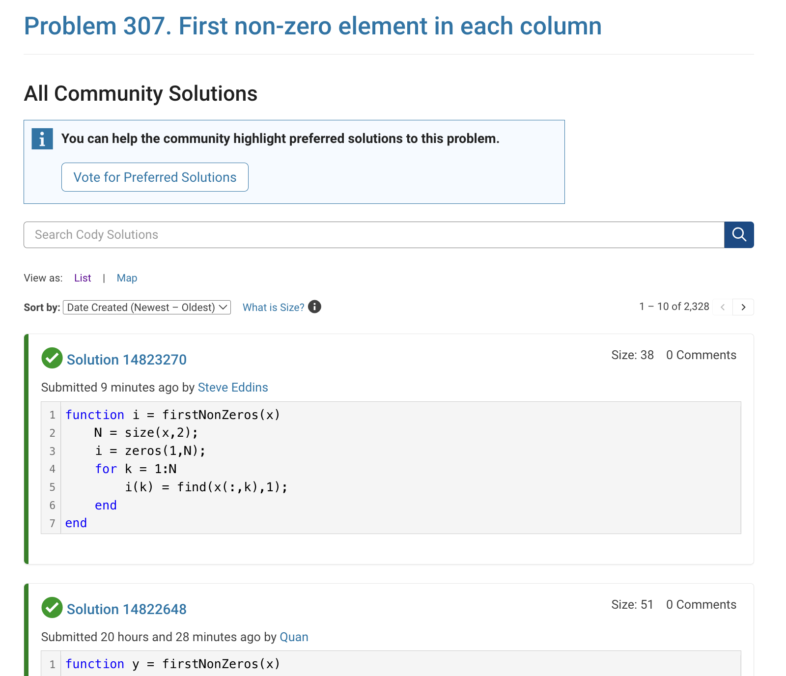
The all-community-solutions view shows the ID of each solution, and you can click on the link to go to the solution.
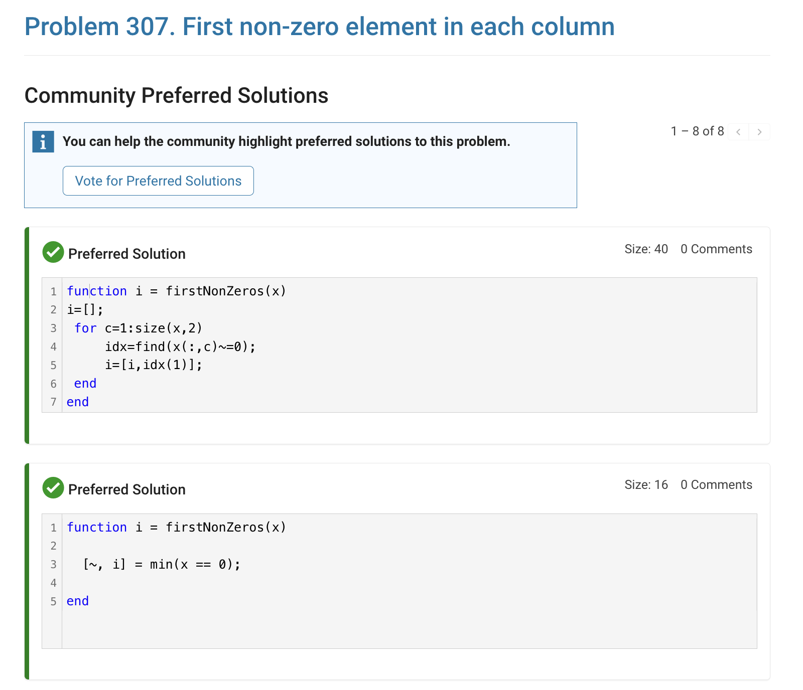
The preferred-community-solutions view does not show the solution IDs and does not link to the solutions. As far as I can tell, there is no way to get from that view to the solutions. If, for example, you want to go to the solution to leave a comment there, you can't.
All-community-solutions view:
Preferred-community-solutions view, with no solution IDs and no links:
Hi cody fellows,
I already solved more than 500 problems -months ago, last july if I remember well- and get this scholar badge, but then it suddenly disappeared a few weeks later. I then solved a few more problems and it reappeared.
Now I observed it disappeared once more a few days ago.
Have you also noticed this erratic behavior of the scholar badge ? Is it normal and / or intentional ? If not, how to explain it ? (deleted problems ?)
Cheers,
Nicolas
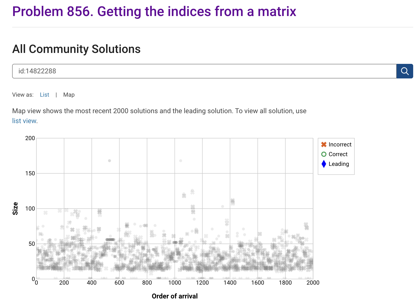
I'm seeing solution maps shown with low-contrast gray colors instead of the correct symbol colors. I have observed this using both Safari and Chrome. Screenshot:
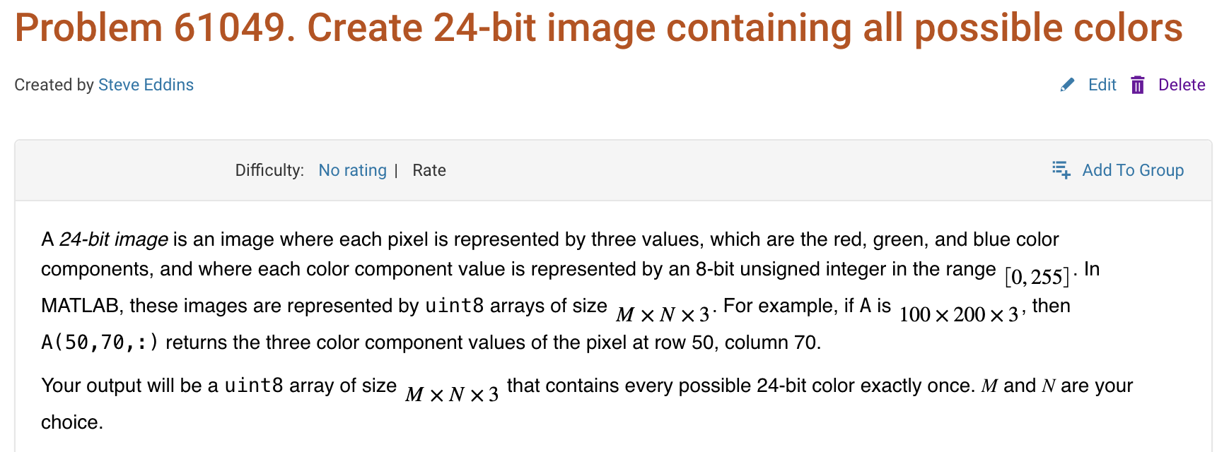
Here is a screenshot of a Cody problem that I just created. The math rendering is poor. (I have since edited the problem to remove the math formatting.)