主要内容
Results for
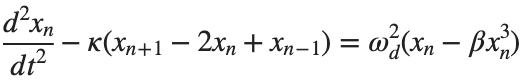
The study of nonlinear dynamical systems in lattices is an area of research with continuously growing interest.The first systematic studies of these systems emerged in the late 1930 s,thanks to the work of Frenkel and Kontorova on crystal dislocations.These studies led to the formulation of the discrete Klein-Gordon equation (DKG).Specifically,in 1939,Frenkel and Kontorova proposed a model that describes the structure and dynamics of a crystal lattice in a dislocation core.The FK model has become one of the fundamental models in physics,as it has been proven to reliably describe significant phenomena observed in discrete media.The equation we will examine is a variation of the following form:

The process described involves approximating a nonlinear differential equation through the Taylor method and simplifying it into a linear model.Let's analyze step by step the process from the initial equation to its final form.For small angles, can be approximated through the Taylor series as:
We substitute  in the original equation with the Taylor approximation:
To map this equation to a linear model,we consider the angles  to correspond to displacements
  in a mass-spring system.Thus,the equation transforms into:
to correspond to displacements We recognize that the term  expresses the nonlinearity of the system,while β is a coefficient corresponding to this nonlinearity,simplifying the expression.The final form of the equation is:
The exact value of β depends on the mapping of coefficients in the Taylor approximation and its application to the specific physical problem.Our main goal is to derive results regarding stability and convergence in nonlinear lattices under nonlinear conditions.We will examine the basic characteristics of the discrete Klein-Gordon equation:
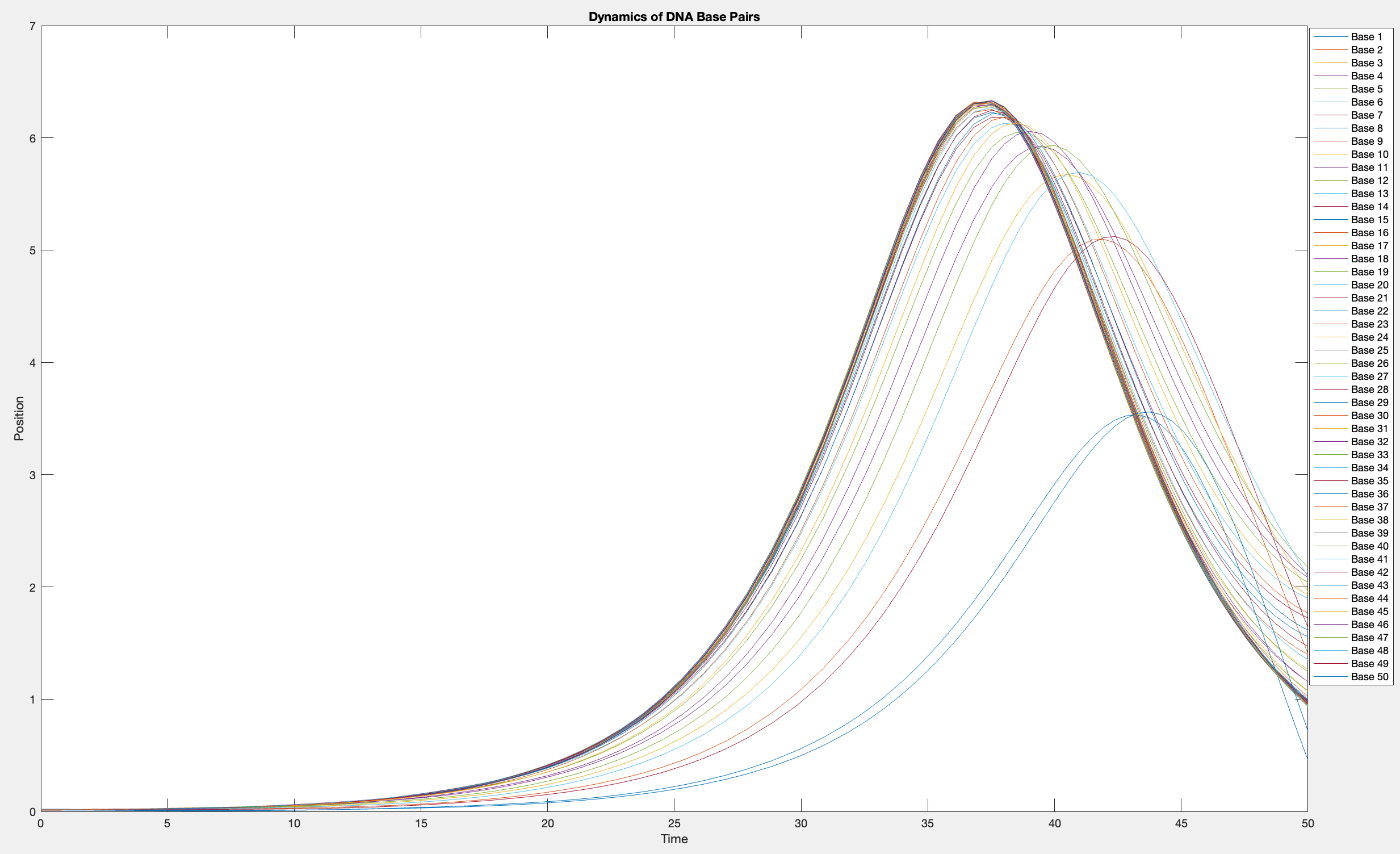
This model is often used to describe the opening of the DNA double helix during processes such as transcription.The model focuses on the transverse motion of the base pairs,which can be represented by a set of coupled nonlinear differential equations.
% Parameters
numBases = 50; % Number of base pairs
kappa = 0.1; % Elasticity constant
omegaD = 0.2; % Frequency term
beta = 0.05; % Nonlinearity coefficient
% Initial conditions
initialPositions = 0.01 + (0.02 - 0.01) * rand(numBases, 1);
initialVelocities = zeros(numBases, 1);
Time span
tSpan = [0 50];
>> % Differential equations
odeFunc = @(t, y) [y(numBases+1:end); ... % velocities
kappa * ([y(2); y(3:numBases); 0] - 2 * y(1:numBases) + [0; y(1:numBases-1)]) + ...
omegaD^2 * (y(1:numBases) - beta * y(1:numBases).^3)]; % accelerations
% Solve the system
[T, Y] = ode45(odeFunc, tSpan, [initialPositions; initialVelocities]);
% Visualization
plot(T, Y(:, 1:numBases))
legend(arrayfun(@(n) sprintf('Base %d', n), 1:numBases, 'UniformOutput', false))
xlabel('Time')
ylabel('Position')
title('Dynamics of DNA Base Pairs')
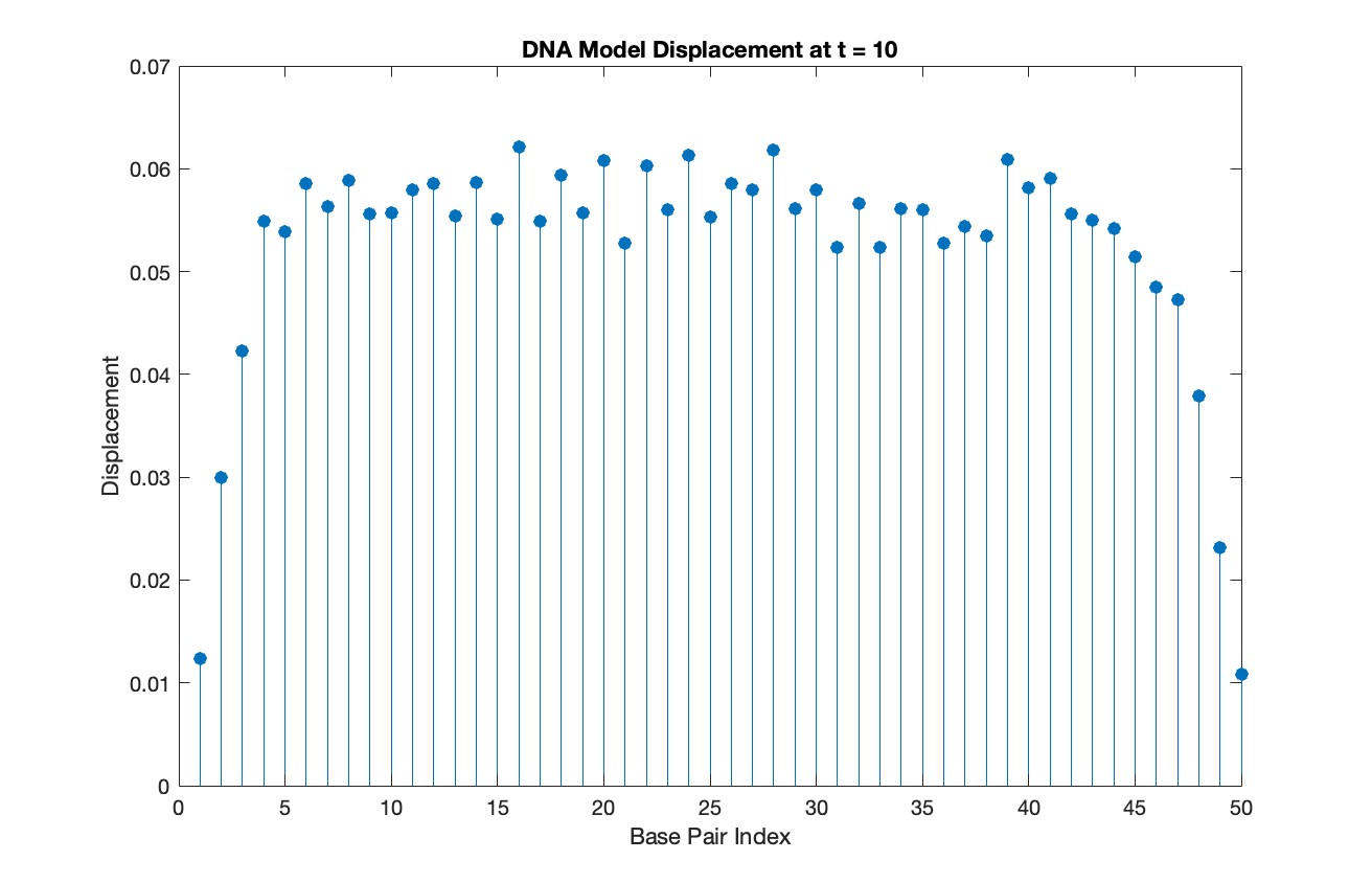
% Choose a specific time for the snapshot
snapshotTime = 10;
% Find the index in T that is closest to the snapshot time
[~, snapshotIndex] = min(abs(T - snapshotTime));
% Extract the solution at the snapshot time
snapshotSolution = Y(snapshotIndex, 1:numBases);
% Generate discrete plot for the DNA model at the snapshot time
figure;
stem(1:numBases, snapshotSolution, 'filled')
title(sprintf('DNA Model Displacement at t = %d', snapshotTime))
xlabel('Base Pair Index')
ylabel('Displacement')
% Time vector for detailed sampling
tDetailed = 0:0.5:50;
% Initialize an empty array to hold the data
data = [];
% Generate the data for 3D plotting
for i = 1:numBases
% Interpolate to get detailed solution data for each base pair
detailedSolution = interp1(T, Y(:, i), tDetailed);
% Concatenate the current base pair's data to the main data array
data = [data; repmat(i, length(tDetailed), 1), tDetailed', detailedSolution'];
end
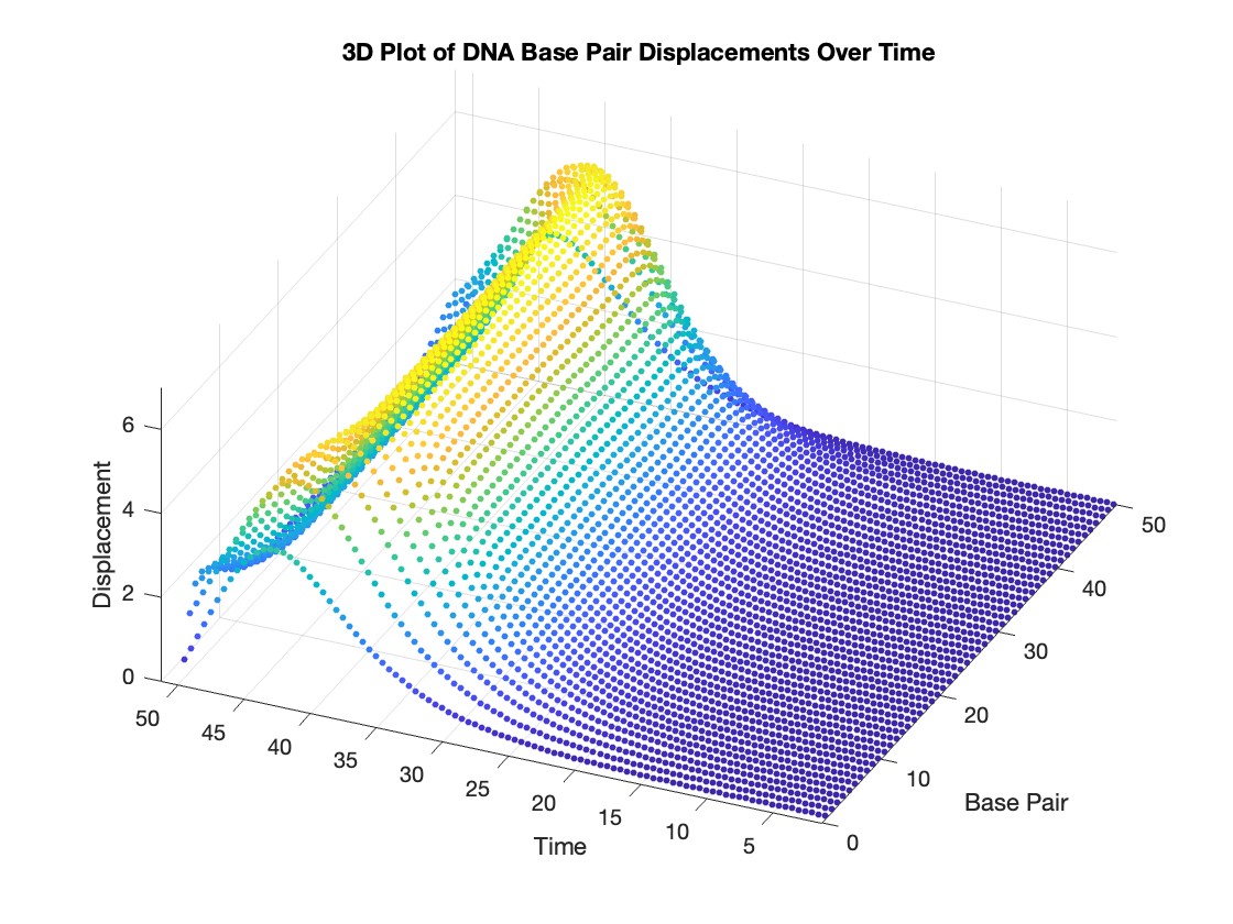
% 3D Plot
figure;
scatter3(data(:,1), data(:,2), data(:,3), 10, data(:,3), 'filled')
xlabel('Base Pair')
ylabel('Time')
zlabel('Displacement')
title('3D Plot of DNA Base Pair Displacements Over Time')
colormap('rainbow')
colorbar
Lots of students like me have a break from school this week or next! If y'all are looking for something interesting to do learn a bit about using hgtransform by making the transforming snake animation in MATLAB!
Code below!
⬇️⬇️⬇️
numblock=24;
v = [ -1 -1 -1 ; 1 -1 -1 ; -1 1 -1 ; -1 1 1 ; -1 -1 1 ; 1 -1 1 ];
f = [ 1 2 3 nan; 5 6 4 nan; 1 2 6 5; 1 5 4 3; 3 4 6 2 ];
clr = hsv(numblock);
shapes = [ 1 0 0 0 0 0 1 0 0 0 0 1 0 0 0 0 0 0 1 0 0 0 0 1 % box
0 0 .5 -.5 .5 0 1 0 -.5 .5 -.5 0 1 0 .5 -.5 .5 0 1 0 -.5 .5 -.5 0 % fluer
0 0 1 1 0 .5 -.5 1 .5 .5 -.5 -.5 1 .5 .5 -.5 -.5 1 .5 .5 -.5 -.5 1 .5 % bowl
0 .5 -.5 -.5 .5 -.5 .5 .5 -.5 .5 -.5 -.5 .5 -.5 .5 .5 -.5 .5 -.5 -.5 .5 -.5 .5 .5]; % ball
% Build the assembly
set(gcf,'color','black');
daspect(newplot,[1 1 1]);
xform=@(R)makehgtform('axisrotate',[0 1 0],R,'zrotate',pi/2,'yrotate',pi,'translate',[2 0 0]);
P=hgtransform('Parent',gca,'Matrix',makehgtform('xrotate',pi*.5,'zrotate',pi*-.8));
for i = 1:numblock
P = hgtransform('Parent',P,'Matrix',xform(shapes(end,i)*pi));
patch('Parent',P, 'Vertices', v, 'Faces', f, 'FaceColor',clr(i,:),'EdgeColor','none');
patch('Parent',P, 'Vertices', v*.75, 'Faces', f(end,:), 'FaceColor','none',...
'EdgeColor','w','LineWidth',2);
end
view([10 60]);
axis tight vis3d off
camlight
% Setup vectors for animation
h=findobj(gca,'type','hgtransform')'; h=h(2:end);
r=shapes(end,:)*pi;
steps=100;
% Animate between different shapes
for si = 1:size(shapes,1)
sh = shapes(si,:)*pi;
diff = (sh-r)/steps;
% Animate to a new shape
for s=1:steps
arrayfun(@(tx)set(h(tx),'Matrix',xform(r(tx)+diff(tx)*s)),1:numblock);
view([s*360/steps 20]); drawnow();
end
r=sh;
for s=1:steps; view([s*360/steps 20]); drawnow(); end % finish rotate
end
Several of the colormaps are great for a 256 color surface plot, but aren't well optimized for extracting m colors for plotting several independent lines. The issue is that many colormaps have start/end colors that are too similar or are suboptimal colors for lines. There are certainly many workarounds for this, but it would be a great quality of life to adjust that directly when calling this.
Example:
x = linspace(0,2*pi,101)';
y = [1:6].*cos(x);
figure; plot(x,y,'LineWidth',2); grid on; axis tight;
And now if I wanted to color these lines, I could use something like turbo(6) or gray(6) and then apply it using colororder.
colororder(turbo(6))
But my issue is that the ends of the colormap are too similar. For other colormaps, you may get lines that are too light to be visible against the white background. There are plenty of workarounds, with my preference being to create extra colors and truncate that before using colororder.
cmap = turbo(8); cmap = cmap(2:end-1,:); % Truncate the end colors
figure; plot(x,y,'LineWidth',2); grid on; axis tight;
colororder(cmap)
I think it would be really awesome to add some name-argument input pair to these colormaps that can specify the range you want so this could even be done inside the colororder calling if desired. An example of my proposed solution would look something like this:
cmap = turbo(6,'Range',[0.1 0.8]); % Proposed idea to add functionality
Where in this scenario, the resulting colormap would be 6 equally spaced colors that range from 10% to 80% of the total color range. This would be especially nice because you could more quickly modify the range of colors, or you could set the limits regardless of whether you need to plot 3, 6, or 20 lines.
I asked my question in the general forum and a few minutes later it was deleted. Perhaps this is a better place?
Rather than using my German regional forum (as I do not speak German), I want to ask questions in an international English-speaking forum. Presumably there should be an international English forum for everyone around the world, as English is the first or second language of everyone who has gone to school. Where is it?
2 x 2 행렬의 행렬식은
- 행렬의 두 row 벡터로 정의되는 평행사변형의 면적입니다.
- 물론 두 column 벡터로 정의되는 평행사변형의 면적이기도 합니다.
- 좀 더 정확히는 signed area입니다. 면적이 음수가 될 수도 있다는 뜻이죠.
- 행렬의 두 행(또는 두 열)을 맞바꾸면 행렬식의 부호도 바뀌고 면적의 부호도 바뀌어야합니다.
일반적으로 n x n 행렬의 행렬식은
- 각 row 벡터(또는 각 column 벡터)로 정의되는 N차원 공간의 평행면체(?)의 signed area입니다.
- 제대로 이해하려면 대수학의 개념을 많이 가지고 와야 하는데 자세한 설명은 생략합니다.(=저도 모른다는 뜻)
- 더 자세히 알고 싶으시면 수학하는 만화의 '넓이 이야기' 편을 추천합니다.
- 수학적인 정의를 알고 싶으시면 위키피디아를 보시면 됩니다.
- 이렇게 생겼습니다. 좀 무섭습니다.
아래 코드는...
- 2 x 2 행렬에 대해서 이것을 수식 없이 그림만으로 증명하는 과정입니다.
- gif 생성에는 ScreenToGif를 사용했습니다. (gif 만들기엔 이게 킹왕짱인듯)
Determinant of 2 x 2 matrix is...
- An area of a parallelogram defined by two row vectors.
- Of course, same one defined by two column vectors.
- Precisely, a signed area, which means area can be negative.
- If two rows (or columns) are swapped, both the sign of determinant and area change.
More generally, determinant of n x n matrix is...
- Signed area of parallelepiped defined by rows (or columns) of the matrix in n-dim space.
- For a full understanding, a lot of concepts from abstract algebra should be brought, which I will not write here. (Cuz I don't know them.)
- For a mathematical definition of determinant, visit wikipedia.

- A little scary, isn't it?
The code below is...
- A process to prove the equality of the determinant of 2 x 2 matrix and the area of parallelogram.
- ScreenToGif is used to generate gif animation (which is, to me, the easiest way to make gif).
% 두 점 (a, b), (c, d)의 좌표
a = 4;
b = 1;
c = 1;
d = 3;
% patch 색 pre-define
lightgreen = [144, 238, 144]/255;
lightblue = [169, 190, 228]/255;
lightorange = [247, 195, 160]/255;
% animation params.
anim_Nsteps = 30;
% create window
figure('WindowStyle','docked')
ax = axes;
ax.XAxisLocation = 'origin';
ax.YAxisLocation = 'origin';
ax.XTick = [];
ax.YTick = [];
hold on
ax.XLim = [-.4, a+c+1];
ax.YLim = [-.4, b+d+1];
% create ad-bc patch
area = patch([0, a, a+c, c], [0, b, b+d, d], lightgreen);
p_ab = plot(a, b, 'ko', 'MarkerFaceColor', 'k');
p_cd = plot(c, d, 'ko', 'MarkerFaceColor', 'k');
p_ab.UserData = text(a+0.1, b, '(a, b)', 'FontSize',16);
p_cd.UserData = text(c+0.1, d-0.2, '(c, d)', 'FontSize',16);
area.UserData = text((a+c)/2-0.5, (b+d)/2, 'ad-bc', 'FontSize', 18);
pause
%% Is this really ad-bc?
area.UserData.String = 'ad-bc...?';
pause
%% fade out ad-bc
fadeinout(area, 0)
area.UserData.Visible = 'off';
pause
%% fade in ad block
rect_ad = patch([0, a, a, 0], [0, 0, d, d], lightblue, 'EdgeAlpha', 0, 'FaceAlpha', 0);
uistack(rect_ad, 'bottom');
fadeinout(rect_ad, 1, t_pause=0.003)
draw_gridline(rect_ad, ["23", "34"])
rect_ad.UserData = text(mean(rect_ad.XData), mean(rect_ad.YData), 'ad', 'FontSize', 20, 'HorizontalAlignment', 'center');
pause
%% fade-in bc block
rect_bc = patch([0, c, c, 0], [0, 0, b, b], lightorange, 'EdgeAlpha', 0, 'FaceAlpha', 0);
fadeinout(rect_bc, 1, t_pause=0.0035)
draw_gridline(rect_bc, ["23", "34"])
rect_bc.UserData = text(b/2, c/2, 'bc', 'FontSize', 20, 'HorizontalAlignment', 'center');
pause
%% slide ad block
patch_slide(rect_ad, ...
[0, 0, 0, 0], [0, b, b, 0], t_pause=0.004)
draw_gridline(rect_ad, ["12", "34"])
pause
%% slide ad block
patch_slide(rect_ad, ...
[0, 0, d/(d/c-b/a), d/(d/c-b/a)],...
[0, 0, b/a*d/(d/c-b/a), b/a*d/(d/c-b/a)], t_pause=0.004)
draw_gridline(rect_ad, ["14", "23"])
pause
%% slide bc block
uistack(p_cd, 'top')
patch_slide(rect_bc, ...
[0, 0, 0, 0], [d, d, d, d], t_pause=0.004)
draw_gridline(rect_bc, "34")
pause
%% slide bc block
patch_slide(rect_bc, ...
[0, 0, a, a], [0, 0, 0, 0], t_pause=0.004)
draw_gridline(rect_bc, "23")
pause
%% slide bc block
patch_slide(rect_bc, ...
[d/(d/c-b/a), 0, 0, d/(d/c-b/a)], ...
[b/a*d/(d/c-b/a), 0, 0, b/a*d/(d/c-b/a)], t_pause=0.004)
pause
%% finalize: fade out ad, bc, and fade in ad-bc
rect_ad.UserData.Visible = 'off';
rect_bc.UserData.Visible = 'off';
fadeinout([rect_ad, rect_bc, area], [0, 0, 1])
area.UserData.String = 'ad-bc';
area.UserData.Visible = 'on';
%% functions
function fadeinout(objs, inout, options)
arguments
objs
inout % 1이면 fade-in, 0이면 fade-out
options.anim_Nsteps = 30
options.t_pause = 0.003
end
for alpha = linspace(0, 1, options.anim_Nsteps)
for i = 1:length(objs)
switch objs(i).Type
case 'patch'
objs(i).FaceAlpha = (inout(i)==1)*alpha + (inout(i)==0)*(1-alpha);
objs(i).EdgeAlpha = (inout(i)==1)*alpha + (inout(i)==0)*(1-alpha);
case 'constantline'
objs(i).Alpha = (inout(i)==1)*alpha + (inout(i)==0)*(1-alpha);
end
pause(options.t_pause)
end
end
end
function patch_slide(obj, x_dist, y_dist, options)
arguments
obj
x_dist
y_dist
options.anim_Nsteps = 30
options.t_pause = 0.003
end
dx = x_dist/options.anim_Nsteps;
dy = y_dist/options.anim_Nsteps;
for i=1:options.anim_Nsteps
obj.XData = obj.XData + dx(:);
obj.YData = obj.YData + dy(:);
obj.UserData.Position(1) = mean(obj.XData);
obj.UserData.Position(2) = mean(obj.YData);
pause(options.t_pause)
end
end
function draw_gridline(patch, where)
ax = patch.Parent;
for i=1:length(where)
v1 = str2double(where{i}(1));
v2 = str2double(where{i}(2));
x1 = patch.XData(v1);
x2 = patch.XData(v2);
y1 = patch.YData(v1);
y2 = patch.YData(v2);
if x1==x2
xline(x1, 'k--')
else
fplot(@(x) (y2-y1)/(x2-x1)*(x-x1)+y1, [ax.XLim(1), ax.XLim(2)], 'k--')
end
end
end
Happy year of the dragon.
I was looking into the possibility of making a spin-to-win prize wheel in MATLAB. I was looking around, and if someone has made one before they haven't shared. A labeled colored spinning wheel, that would slow down and stop (or I would take just stopping) at a random spot each time. I would love any tips or links to helpful resources!
Many of the examples in the MATLAB documentation are extremely high quality articles, often worthy of attention in their own right. Time to start celebrating them! Today's is how to increase Image Resolution using deep learning
https://uk.mathworks.com/help/deeplearning/ug/single-image-super-resolution-using-deep-learning.html
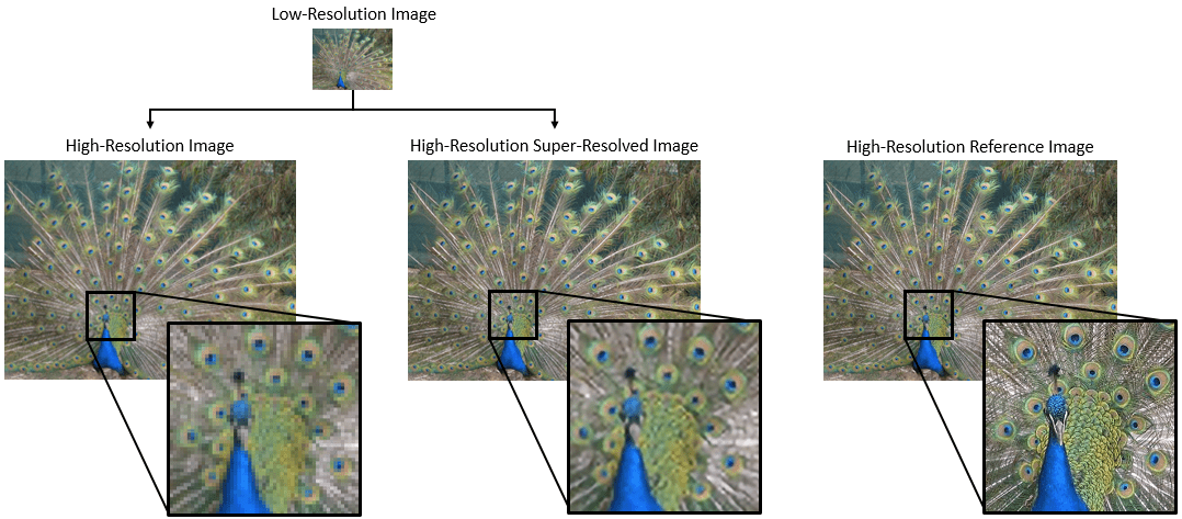
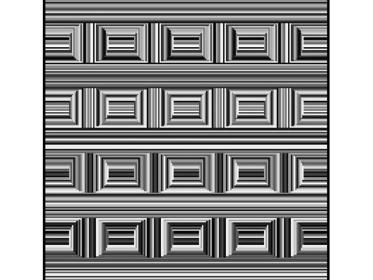
Can you see them?
I have been procrastinating on schoolwork by looking at all the amazing designs created in the last MATLAB Flipbook Mini Hack! They are just amazing. The voting is over but what are y'all's personal favorites? Mine is the flapping butterfly, it is for sure a creation I plan to share with others in the future!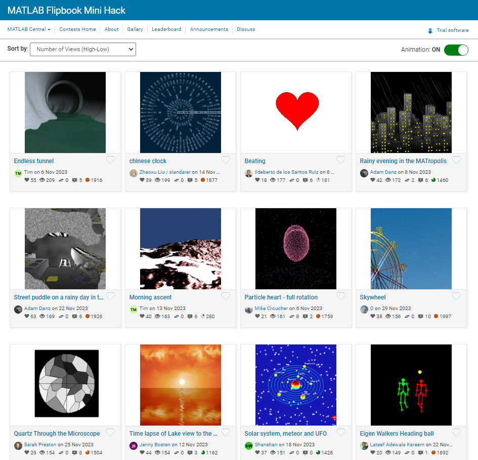
Struct is an easy way to combine different types of variants. But now MATLAB supports classes well, and I think class is always a better alternative than struct. I can't find a single scenario that struct is necessary. There are many shortcomings using structs in a project, e.g. uncontrollable field names, unexamined values, etc. What's your opinion?
I am confused, is the matlab answer better or Julia’s?
Hello and a warm welcome to all! We're thrilled to have you visit our community. MATLAB Central is a place for learning, sharing, and connecting with others who share your passion for MATLAB and Simulink. To ensure you have the best experience, here are some tips to get you started:
- Read the Community Guidelines: Understanding our community standards is crucial. Please take a moment to familiarize yourself with them. Keep in mind that posts not adhering to these guidelines may be flagged by moderators or other community members.
- Ask Technical Questions at MATLAB Answers: If you have questions related to MathWorks products, head over to MATLAB Answers (new question form - Ask the community). It's the go-to spot for technical inquiries, with responses often provided within an hour, depending on the complexity of the question and volunteer availability. To increase your chances of a speedy reply, check out our tips on how to craft a good question (link to post on asking good questions).
- Choosing the Right Channel: We offer a variety of discussion channels tailored to different contexts. Select the one that best fits your post. If you're unsure, the General channel is always a safe bet. If you feel there's a need for a new channel, we encourage you to suggest it in the Ideas channel.
- Reporting Issues: If you encounter posts that violate our guidelines, please use the 🚩Flag/Report feature (found in the 3-dot menu) to bring them to our attention.
- Quality Control: We strive to maintain a high standard of discussion. Accounts that post spam or too much nonsense may be subject to moderation, which can include temporary suspensions or permanent bans.
- Share Your Ideas: Your feedback is invaluable. If you have suggestions on how we can improve the community or MathWorks products, the Ideas channel is the perfect place to voice your thoughts.
Enjoy yourself and have fun! We're committed to fostering a supportive and educational environment. Dive into discussions, share your expertise, and grow your knowledge. We're excited to see what you'll contribute to the community!
Have you ever used Live Tasks in MATLAB? MathWorks development team would like to get some feedback on your experience – what did you like and not like. Especially, if you know about it but don’t use it frequently, we would like to understand why?
Please tell us what you think by submitting your response to this form https://forms.office.com/r/ui1EGqAFDx
One of my colleauges, Michio, recently posted an implementation of Pong Wars in MATLAB
- Here's the code on GitHub.https://lnkd.in/gZG-AsFX
- If you want to open with MATLAB Online, click here https://lnkd.in/gahrTMW5
- He saw this first here: https://lnkd.in/gu_Z-Pks
Making me wonder about variations. What might the resulting patterns look with differing numbers of balls? Different physics etc?
MathWorks just released three new courses on Coursera liseted below. If you work with image or video data and are wanting to incorporate deep learning techniques into your workflow, this is a great opporutnity. The course creators monitor the discussion forums, so you can ask questions and get feedback on your work. Below are links to the three courses and a quick description of a project you'll complete in each.
- Introduction to Computer Vision for Deep Learning. You'll train a classifier to classify images of people signing the American Sign Language alphabet.
- Deep Learning for Object Detection. Move from just classification to finding object locations. You'll train a model to find different types of parking available on the MathWorks campus.
- Advanced Deep Learning Techniques for Computer Vision. You'll train anomaly detection models for medical images and use AI-assisted labeling auto label images.
Can anyone provide insight into the intended difference between Discussions and Answers and what should be posted where?
Just scrolling through Discussions, I saw postst that seem more suitable Answers?
What exactly does Discussions bring to the table that wasn't already brought by Answers?
Maybe this question is more suitable for a Discussion ....
Hello Community!
We are working on a new translation experience for the MathWorks website and products. The goal is to make it easy for people to see content in the best language for them.
Step 1 is learning from those of you who use another language instead of, or in addition to English. If this sounds like you, we'd love your response to a brief survey.
Feel free to comment here as well. Thanks in advance!
We've released an open-source implementation of STIPA (Speech Transmission Index for Public Address) on GitHub!
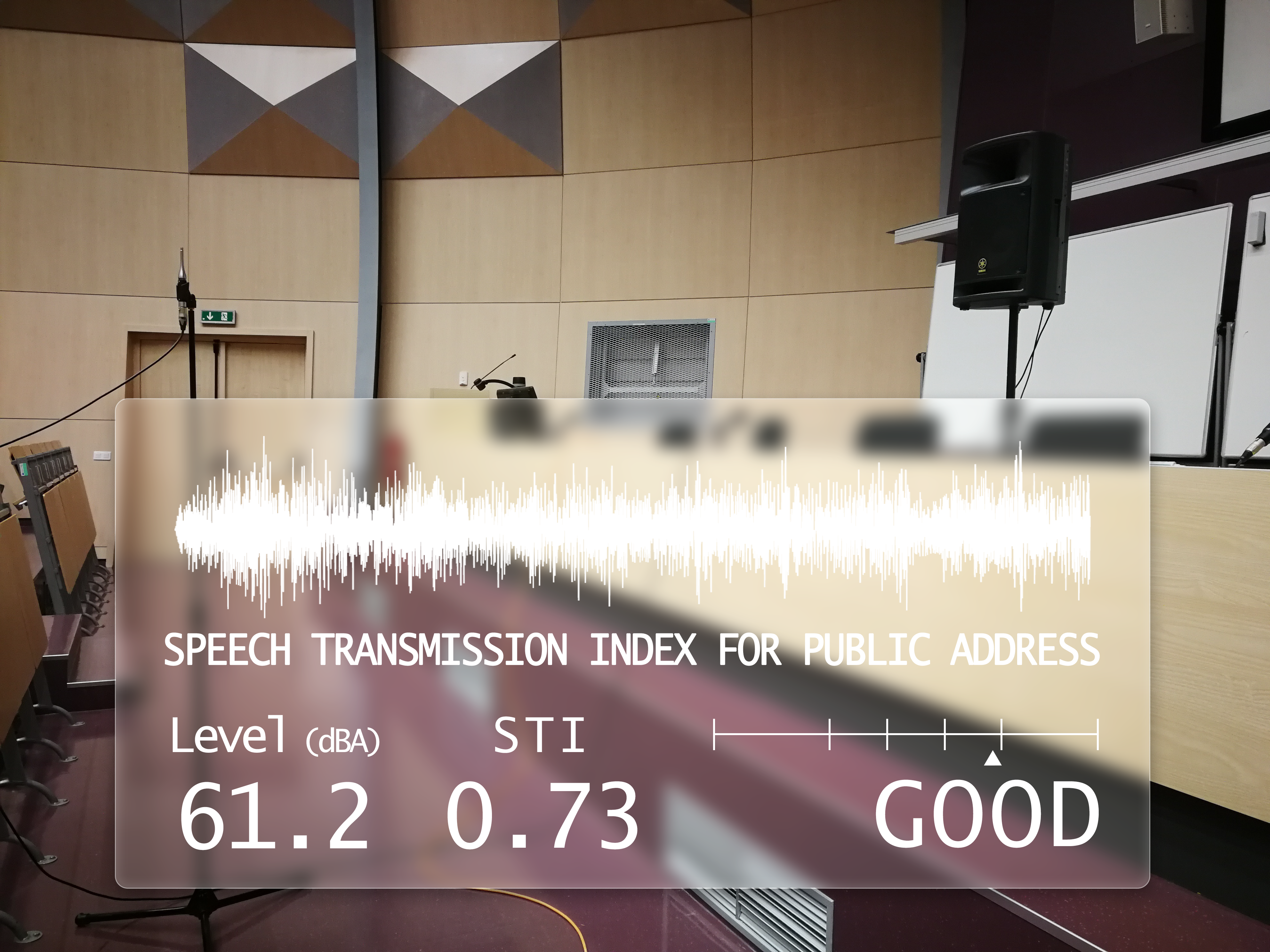
What is STIPA?
Speech Transmission Index is a metric designed to assess the quality of speech transmission through a communication channel. It quantifies the intelligibility of speech signals based on amplitude modulations, providing a standardized measure crucial for evaluating public address systems and communication equipment. STIPA is a version of STI using a simplified measurement method and only one test signal.
Quality Representation:
STI values range from 0 to 1, categorizing speech transmission quality from bad to excellent. The raw STI score can be transformed into the likelihood of intelligibility of syllables, words, and sentences being comprehended.
Verification Tests:
To ensure reliability, we've conducted verification tests according to the IEC 60286-16 standard. Download the test signals and run the stipaVerificationTests.m script from our GitHub repository.
Control Measurements:
We've performed comparative measurements in a university auditorium, showcasing the validity of our implementation.
License:
Our STIPA implementation is distributed under the GNU General Public License 3, reflecting our commitment to open-source collaboration.

您也可以从以下列表中选择网站:
美洲
- América Latina (Español)
- Canada (English)
- United States (English)
欧洲
- Belgium (English)
- Denmark (English)
- Deutschland (Deutsch)
- España (Español)
- Finland (English)
- France (Français)
- Ireland (English)
- Italia (Italiano)
- Luxembourg (English)
- Netherlands (English)
- Norway (English)
- Österreich (Deutsch)
- Portugal (English)
- Sweden (English)
- Switzerland
- United Kingdom(English)
亚太
- Australia (English)
- India (English)
- New Zealand (English)
- 中国
- 日本Japanese (日本語)
- 한국Korean (한국어)