主要内容
搜索
At the present time, the following problems are known in MATLAB Answers itself:
- Symbolic output is not displaying. The work-around is to disp(char(EXPRESSION)) or pretty(EXPRESSION)
- Symbolic preferences are sometimes set to non-defaults
I was curious to startup your new AI Chat playground.
The first screen that popped up made the statement:
"Please keep in mind that AI sometimes writes code and text that seems accurate, but isnt"
Can someone elaborate on what exactly this means with respect to your AI Chat playground integration with the Matlab tools?
Are there any accuracy metrics for this integration?
Just shared an amazing YouTube video that demonstrates a real-time PID position control system using MATLAB and Arduino.
I don't like the change
16%
I really don't like the change
29%
I'm okay with the change
24%
I love the change
11%
I'm indifferent
11%
I want both the web & help browser
11%
38 个投票

You can make a lot of interesting objects with matlab primitive shapes (e.g. "cylinder," "sphere," "ellipsoid") by beginning with some of the built-in Matlab primitives and simply applying deformations. The gif above demonstrates how the Manta animation was created using a cylinder as the primitive and successively applying deformations: (https://www.mathworks.com/matlabcentral/communitycontests/contests/8/entries/16252);
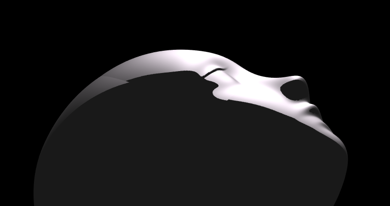
Similarly, last year a sphere was deformed to create a face in two of my submissions, for example, the profile in "waking":
You can piece-wise assemble images, but one of the advantages of creating objects with deformations is that you have a parametric representation of the surface. Creating a higher or lower polygon rendering of the surface is as simple as declaring the number of faces in the orignal primitive. For example here is the scene in "snowfall" using sphere with different numbers of input faces:
sphere(100)
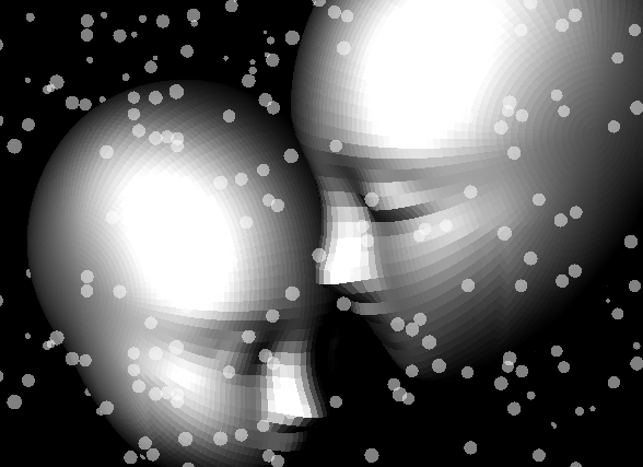
sphere(500)
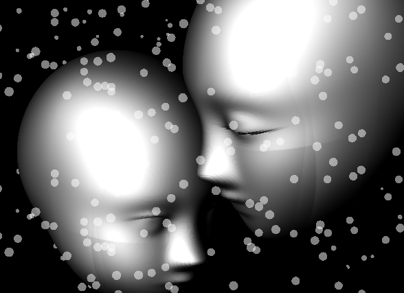
High poly models aren't always better. Low-polygon shapes can sometimes add a little distance from that low point in the uncanny valley.
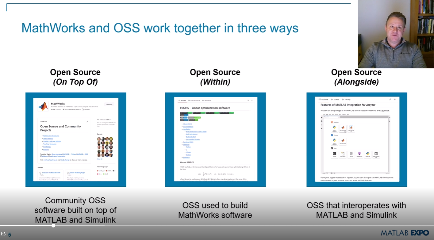
Next week is MATLAB EXPO week and it will be the first one that I'm presenting at! I'll be giving two presentations, both of which are related to the intersection of MATLAB and open source software.
- Open Source Software and MATLAB: Principles, Practices, and Python Along with MathWorks' Heather Gorr. We we discuss three different types of open source software with repsect to their relationship to MATLAB
- The CLASSIX Story: Developing the Same Algorithm in MATLAB and Python Simultaneously A collaboration with Prof. Stefan Guettel from University of Manchester. Developing his clustering algorithm, CLASSIX, in both Python and MATLAB simulatenously helped provide insights that made the final code better than if just one language was used.
There are a ton of other great talks too. Come join us! (It's free!) MATLAB EXPO 2024
Hi MATLAB Central community! 👋
I’m currently working on a project where I’m integrating MATLAB analytics into a mobile app, mainly to handle data-heavy tasks like processing sensor data and running predictive models. The app is built for Android, and while it’s not entirely MATLAB-based, I use MATLAB for a lot of data preprocessing and model training.
I wanted to reach out and see if anyone else here has experience with using MATLAB for similar mobile or embedded applications. Here are a few areas I’m focusing on:1. Optimizing MATLAB Code for Mobile Compatibility
I’ve found that some MATLAB functions work perfectly on desktop but may run slower or encounter limitations on mobile. I’ve tried using code generation and reducing function calls where possible, but I’m curious if anyone has other tips for optimizing MATLAB code for mobile environments?
2. Using MATLAB for Sensor Data Processing
I’m working with accelerometer and GPS data, and MATLAB has been great for preprocessing. However, I wonder if anyone has suggestions for handling large sensor datasets efficiently in MATLAB, especially if you've managed data in mobile contexts?
3. Integrating MATLAB Models into Mobile Apps
I’ve heard about using MATLAB Compiler SDK to integrate MATLAB algorithms into other environments. For those who have done this, what’s the best way to maintain performance without excessive computational strain on the device?
4. Data Visualization Tips
Has anyone had experience with mobile-friendly data visualizations using MATLAB? I’ve been using basic plots, but I’d love to know if there are any resources or toolboxes that make it easier to create lightweight, interactive visuals for mobile.
If anyone here has tips, tools, or experiences with MATLAB in mobile development, I’d love to hear them! Thanks in advance for any advice you can share!
Go to this page, scroll down to the middle of the long page where you see "Coding Photo editing STEM Business ...." and select "STEM". Voilà!
Mini Hack is brilliant!Let's use MATLAB to create the future!
Pumpkins have been a popular, recurring, and ever-evolving theme in MATLAB during the past few years, and particularly during this time of year. Much of this is driven by the epic work of @Eric Ludlam and expanded upon by many others. The list of material is too extensive to go through everything individually, but I'm listing some of my favourite resources below and I highly recommend these to everyone as they're a lot of fun to play with:
Pumpkins are also particularly prominent during the yearly Mini Hack Contests. This year, I have jumped onto the bandwagon myself with my Floating Pumpkins entry:
In this post, I would like to introduce the concept of masking 3D surfaces in a festive and fun way, by showcasing how to apply it for carving faces on pumpkins step by step.
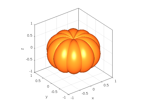
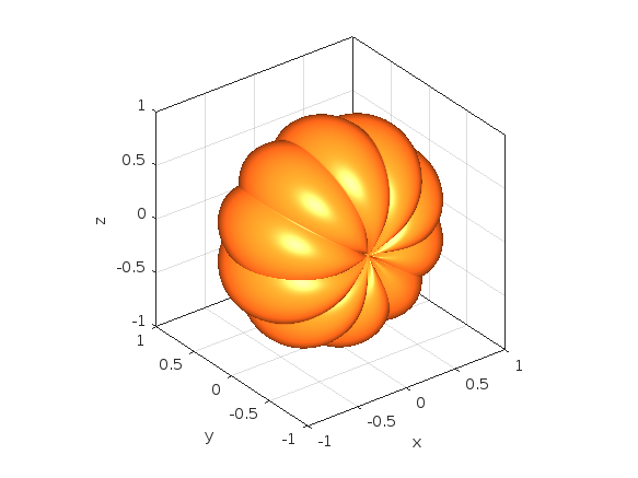
Let's start by drawing the pumpkin's body. The following was adapted from Eric's code:
n = 600; % Number of faces
% Shape pumpkin's rind (skin)
[X,Y,Z] = sphere(n);
% Shape pumpkin's ribs (ridges)
R = (1-(1-mod(0:20/n:20,2)).^2/12);
X = X.*R; Y = Y.*R; Z = Z.*R;
Z = (.8+(0-linspace(1,-1,n+1)'.^4)*.3).*Z;
function plotPumpkin(X,Y,Z)
figure
surf(X,Y,Z,'FaceColor',[1 .4 .1],'EdgeColor','none');
hold on
box on
axis([-1 1 -1 1 -1 1],'square')
xlabel('x'); xticks(-1:0.5:1)
ylabel('y'); yticks(-1:0.5:1)
zlabel('z'); zticks(-1:0.5:1)
material([.45,.7,.25])
camlight('headlight')
camlight('headlight')
lighting gouraud
end
plotPumpkin(X,Y,Z)
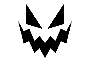
The next step is drawing the face for the mask. This can be done in 2D and can consist of any number of lines that form polygonal closed shapes and are appropriately scaled relative to the coordinates of the pumpkin. A quick example:
% Mouth
xm = [-.5:.1:.5 flip(-.5:.1:.5)];
ym = [.15 -.3 -.25 -.5 -.4 -.6 flip([.15 -.3 -.25 -.5 -.4]) .15 -.05 0 -.25 -.15 -.3 flip([.15 -.05 0 -.25 -.15])];
% Right eye
xr = [-.35 -.05 -.35];
yr = [.1 0 .5];
% Left eye
xl = abs(xr);
yl = yr;
figure('Color','w')
set(gcf,'Position',get(gcf,'Position')/2)
axes('Visible','off','NextPlot','Add')
axis tight square
fill(xm,ym,'k')
fill(xr,yr,'k')
fill(xl,yl,'k')
We then need to apply the 2D mask to the 3D surface. To do that, we project it onto the intersections of the surface with the XY plane. However, as we need the face to appear on the side of the pumpkin, we first need to rotate the pumpkin so that the front side is facing upwards. Essentially, we need to rotate the pumpkin around the x-axis by -π/2 rad.
Let's do this from first principles to better understand the process:
theta = [-pi/2,0,0];
[X,Y,Z] = xyzRotate(X,Y,Z,theta);
function [X,Y,Z] = xyzRotate(X,Y,Z,theta)
% Rotation matrices
Rx = [1 0 0;0 cos(theta(1)) -sin(theta(1));0 sin(theta(1)) cos(theta(1))];
Ry = [cos(theta(2)) 0 sin(theta(2));0 1 0;-sin(theta(2)) 0 cos(theta(2))];
Rz = [cos(theta(3)) -sin(theta(3)) 0;sin(theta(3)) cos(theta(3)) 0;0 0 1];
for i=1:size(X,1)
for j=1:size(X,2)
r=Rx*Ry*Rz*[X(i,j);Y(i,j);Z(i,j)];
X(i,j)=r(1);
Y(i,j)=r(2);
Z(i,j)=r(3);
end
end
end
More information about these transformations can be found here:
When plotting we get:
plotPumpkin(X,Y,Z)
Note that as we have only rotated this around the x-axis, Ry and Rz are equal to eye(3).
We can now apply the mask as discussed. We do this by using one of my favourite functions inpolygon. This gives us the corresponding indices of all the data points located inside our polygonal regions. At this stage, it's important to keep the following in mind:
- The number of faces (n) controls the discretization of the pumpkin. The larger it is, the smoother the mask will be, but at the same time the computational cost will also increase. If you are using this for the contest which has a timeout limit of 235 seconds, you might need to adjust it accordingly.
- You will also need to restrict the Z-coordinates appropriately (Z>=0) so that the mask is only applied on the front side of the pumpkin.
- If you are animating the face mask (more information about this below), and you need the eyes and mouth to fully close at any point, avoid using the second argument of the inpolygon function that gives you the points located on the edge of the regions.
The masking function is given below:
function [X,Y,Z] = Mask(X,Y,Z,xm,ym,xr,yr,xl,yl)
mask = ones(size(Z));
mask((inpolygon(X,Y,xm,ym)|inpolygon(X,Y,xr,yr)|inpolygon(X,Y,xl,yl))&Z>=0) = NaN;
Z = Z.*mask;
end
Applying the mask gives us:
[X,Y,Z]=Mask(X,Y,Z,xm,ym,xr,yr,xl,yl);
plotPumpkin(X,Y,Z)
arrayfun(@(x)light('style','local','position',[0 0 0],'color','y'),1:2)
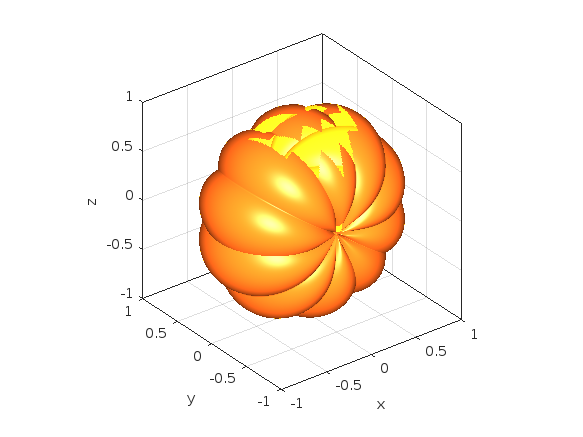
We can see that MATLAB was thoughtful enough to automatically remove the pulp from inside the pumpkin, proving its convenience time and time again.
We can then rotate the pumpkin back and add the stem to get the final result:
theta = [pi/2,0,0];
[X,Y,Z] = xyzRotate(X,Y,Z,theta);
% Stem
s = [1.5 1 repelem(.7, 6)] .* [repmat([.1 .06],1,round(n/20)) .1]';
[t,p] = meshgrid(0:pi/15:pi/2,linspace(0,pi,round(n/10)+1));
Xs = repmat(-(.4-cos(p).*s).*cos(t)+.4,2,1);
Ys = [-sin(p).*s;sin(p).*s];
Zs = repmat((.5-cos(p).*s).*sin(t)+.55,2,1);
plotPumpkin(X,Y,Z)
arrayfun(@(x)light('style','local','position',[0 0 0],'color','y'),1:2)
surf(Xs,Ys,Zs,'FaceColor','#008000','EdgeColor','none');
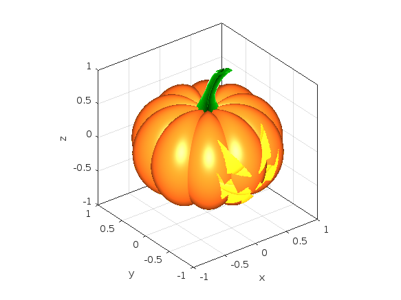
And that's it. You can now add some change to the mask's coordinates between frames and play around with the lighting to get results such as these (more information on how to do this on my Teaser entry):

I hope you have found this tutorial useful, and I'm looking forward to seeing many more creative entries during the final week of the contest.
At the onset of each week, I release a post that analyzes code with the intent of making it accessible for beginners, while also providing insights that can benefit more experienced users seeking to learn new techniques or approaches.
This week, my inspiration comes from the fractal art produced in MATLAB, as presented in my entry Whispers of the Ocean's Breeze:
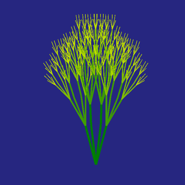
Below, I offer a pretty detailed walkthrough of the code break-down, with the goal of creating both an educational and stimulating experience for those eager to learn or find some inspiration. Taking into account that this post is somewhat lengthy, it provides a breakdown and summary of various techniques. It is my hope that it will assist someone and allow readers to focus on the sections that are of most interest to them.
While the code contains comments, this post offers additional explanations and details.
1. Function Definition and Metadata
function drawframe(f)
Line 1: Defines the main function drawframe, which takes a single parameter f. This parameter controls various aspects of the animation, such as movement or speed.
% Audio source: Klapa Šibenik (comp. Arsen Dedić) -
% - Zaludu me svitovala mati
% (Hrvatska 🇭🇷, (Dalmacija))
% Enhanced aesthetics and added dynamic movement,
% offering a creative Remix of my earlier concept.
% (This version brings richer visual appeal,smoother transitions,
% and a more engaging animation flow)
Lines 2-4: Commented-out lines providing metadata or notes about the code. These comments describe the aesthetic goals and improvements in this version, highlighting that it's a remix of one of my earlier entry's, with added dynamic movement and smoother visuals. (These notes are not executed by MATLAB.)
A general tip for using comments: include comments in your code as frequently as needed. They serve as helpful reminders of what each part of the code does, especially when you revisit it after some time, and make it easier for others who may read or use your code.
2. Function Call to seaweed
seaweed(4) % The value in brackets can be adjusted for significantly
% enhanced visualization,
% but it exceeds the 235-second limit in the contest script.
% Feel free to experiment at Desktop workstation - with higher
% values in the loop,
% for more complex and beautiful results.
Line 5: Calls the seaweed function with an argument of 4. The number 4 controls the recursion depth, affecting how detailed or complex the 'seaweed' pattern will be.
Lines 6-9: Comment explaining that increasing the value in seaweed(4) enhances visualization but may exceed time limits in contest environment(s). This suggests adjusting this parameter on a desktop to explore more intricate patterns...
3. Definition of seaweed Function
function seaweed(k)
% Set up the figure window with a specific position and background color
figure('Position', [60+2*f, 60-2*f, 600, 600], 'Color', [0.15, 0.15, 0.5]);
Line 10: Defines the seaweed function, which takes a parameter k (depth of recursion). This function initializes the graphical figure window.
Line 12: Sets up the figure window with a position influenced by f, making the figure’s position change dynamically with f. The background color [0.15, 0.15, 0.5] creates a dark blue background, enhancing the underwater aesthetic.
4. Recursive Drawing with crta Function
crta([0, 0], 90, k, k);
% Make the axes equal and turn them off for a clean figure
axis equal
axis off
Line 14: Calls the recursive function crta, starting the drawing process at [0, 0](origin point) with a 90-degree angle. Both k values set the initial recursion depth and maximum recursion level.
Lines 16-17: Sets the axis scale to equal, ensuring no distortion, and turns off the axes for a cleaner display.
5. Definition of crtaFunction and Initialization of Parameters
function crta(tck, ugao, prstiter, r)
% Define thickness of line segment proportional to current depth
sir = 5 * (prstiter / r);
% Define length of the line segment
duz1 = 5 * prstiter;
Line 18: Defines crta, a nested function within seaweed, taking parameters tck (current coordinates), ugao (angle), prstiter (current recursion depth), and r (maximum recursion depth).
Lines 20-21: Defines sir (line thickness) to be proportional to the current recursion depth, prstiter, creating thinner branches as depth increases. While, duz1 defines the line segment length, which shortens with each recursion, creating perspective.
6. Angle Calculations for Branching
% Define four branching angles with slight variations
ug1 = ugao + 15 + (f / 15);
ug2 = ugao + 7 - f / 15;
ug3 = ugao - 7 + f / 15;
ug4 = ugao - 15 - f / 15;
Lines 23-27: Sets branching angles ug1, ug2, ug3, and ug4 relative to the initial angle ugao, adding and subtracting small amounts. These angles, influenced by f, introduce subtle variations, enhancing the natural appearance.
7. Calculations for Branch Endpoints
% Calculate endpoints of each line segment for the four angles
a1 = duz1 * sind(ug1) + tck(2);
b1 = duz1 * cosd(ug1) + tck(1);
c2 = duz1 * sind(ug2) + tck(2);
a2 = duz1 * cosd(ug2) + tck(1);
b3 = duz1 * sind(ug3) + tck(2);
c3 = duz1 * cosd(ug3) + tck(1);
d4 = duz1 * sind(ug4) + tck(2);
e4 = duz1 * cosd(ug4) + tck(1);
Lines 29-36: Calculates x and y endpoints for each of the four branches using sind and cosd functions, which convert angles into coordinates. Each branch starts at tck(current In this section, the code calculates the endpoints of four line segments, each corresponding to a distinct angle (ug1, ug2,ug3, and ug4). These endpoints are computed based on the length of the line segment duz1, which scales with recursion depth to make each segment shorter as the recursive function progresses. The trigonometric functions sind and cosd are used here to calculate the horizontal and vertical displacements of each segment relative to the current position, tck. While, sind and cosd functions compute the sine and cosine of each angle in degrees, returning the y and x displacements, respectively. For each angle, multiplying by duz1scales these displacements to achieve the intended length for each line segment. Each endpoint coordinate is calculated by adding these displacements to the initial position, tck, to determine the final position for each branch segment:
- a1 and b1 represent the y and x endpoints for the segment at angle ug1
- c2 and a2 represent the y and x endpoints for the segment at angle ug2
- b3 and c3 represent the y and x endpoints for the segment at angle ug3
- d4 and e4 represent the y and x endpoints for the segment at angle ug4
These coordinates form the four main branches radiating out from the current position in different directions. By varying the angle slightly for each branch and scaling the length proportionally, the function generates a visually rich, organic branching structure that resembles seaweed or other natural patterns.
8. Midpoint Calculations for Additional Complexity
% Calculate midpoints for additional "leaves" to
% simulate complexity
uga1 = ug2 - 5 + f / 5;
ugb2 = ug3 + 5 - f / 5;
uga2 = duz1 / 2 * sind(uga1) + c2 + f / 20;
ugb3 = duz1 / 2 * cosd(uga1) + a2 - f / 20;
ugc2 = duz1 / 2 * sind(ugb2) + b3 + f / 20;
ugda1 = duz1 / 2 * cosd(ugb2) + c3 - f / 20;
Lines 38-44: Calculates midpoint angles and positions for extra “leaf” structures. This further enhances the fractal appearance by adding more detail, as these points fall between main branches!
Additional midpoints are calculated to add further detail and complexity to the fractal pattern. These midpoints represent extra branches or “leaves” that emerge from within the main branch segments, enhancing the natural, organic appearance of the fractal structure. Consequently, uga1 and ugb2 are new angles derived by slightly modifying the main branch angles ug2and ug3. The adjustments are made by adding and subtracting small values, including a component based on f. These subtle variations create slight deviations in the angles of the additional branches, making them appear more random and organic, like leaves growing off main stems in varied directions. Once the new angles uga1 and ugb2 are defined, they are used to calculate intermediate coordinates along the main branch lines. These midpoints are positioned halfway along each branch segment, representing the location from which the extra “leaf” branches will emerge.
To find these midpoints:
- uga2 and ugb3 use sind(uga1) and cosd(uga1)to calculate the y and x coordinates halfway along the segment for angle ug2.
- ugc2 and ugda1 similarly use sind(ugb2) and cosd(ugb2) to get the coordinates for angle ug3.
Each midpoint calculation also includes a slight additional offset based on f (like f / 20), adding variation in their positions and contributing to the irregular, natural look of the structure.
By adding these secondary branches, the fractal pattern gains more intricacy. These “leaves” give a more complex and dense appearance, resembling the growth patterns of plants or seaweed where smaller branches diverge from main stems. The addition of midpoints also contributes to the overall depth and richness of the fractal design, ensuring that each recursive call doesn’t simply repeat but also grows in visual detail, making the resulting fractal more visually appealing and realistic. The midpoint calculations thus play a crucial role in enhancing the visual complexity of the fractal by introducing smaller, secondary branches that break up the regularity of the main branches, making the structure more detailed and lifelike.
9. Color Definition Based on Depth
% Define color based on depth, simulating a gradient effect
% as recursion deepens
boja = [1 - (prstiter / r), 1 - 0.5 * (prstiter / r), 0];
Line 46: Defines the color boja as a gradient that shifts from yellow to dark orange based on recursion depth. This gradient effect enhances the visual depth of the pattern.
This code sets up a color gradient for each branch segment based on its recursion depth. This approach not only adds aesthetic appeal but also visually separates different levels of recursion, making it easier to perceive depth within the fractal. The variable boja is an RGB color array, where each element represents the intensity of red, green, and blue respectively, on a scale from 0 (no intensity) to 1(full intensity).
The first element, 1 - (prstiter / r), controls the red component. The second element, 1 - 0.5 * (prstiter / r), controls the green component. The third element is set to 0, meaning there is no blue in the color, resulting in a gradient that shifts from yellow (where both red and green are high) to darker orange and then brownish tones as recursion deepens. The color gradually shifts from a bright yellowish tone at shallow recursion levels to a darker, warmer orange as recursion depth increases. This is achieved by gradually decreasing the red and green components of the color as prstiter (current recursion depth) approaches r (maximum recursion depth). At the top levels of recursion (where prstiter is closer to r), the color becomes darker and more subdued, giving the branches a gradient that makes the structure look natural and complex. This effect is reminiscent of how colors in nature tend to fade or darken with distance or depth, such as in underwater scenes where light penetration decreases with depth.
The gradient serves as a visual cue that helps distinguish between different recursion levels. Since each level is progressively darker, viewers can intuitively sense the depth of each branch, which adds to the three-dimensional effect of the fractal. The use of warm colors (yellow to orange) for each branch segment helps the fractal pattern stand out vividly against the cool blue background set in the seaweed function. This color contrast enhances the underwater, organic look of the structure, making it appear as though the "seaweed" is reaching out toward a light source above. This coloring strategy also contributes to the fractal’s aesthetic complexity. By associating color depth with recursion depth, the fractal appears to have layers, creating a visually satisfying and realistic effect.
10. Plotting Branch Segments
% Plot main branches from the starting point (tck) to the calculated
% endpoints with color and transparency
p1 = plot([tck(1), b1], [tck(2), a1], 'LineWidth', sir, 'Color', boja);
hold on
s2 = plot([tck(1), a2], [tck(2), c2], 'LineWidth', sir, 'Color', boja);
s3 = plot([tck(1), c3], [tck(2), b3], 'LineWidth', sir, 'Color', boja);
s4 = plot([tck(1), e4], [tck(2), d4], 'LineWidth', sir, 'Color', boja);
% Plot secondary branches connecting midpoints for added detail
s5 = plot([a2, ugb3], [c2, uga2], 'LineWidth', sir, 'Color', boja);
s6 = plot([c3, ugda1], [b3, ugc2], 'LineWidth', sir, 'Color', boja);
Lines 48-56: Plots the main branches and secondary branches for added detail. Each plot command connects points with a specified thickness and color, creating the branching effect.
Here presented code, plots the main branches and additional “leaf” segments, giving form to the fractal pattern. Each plot command specifies a line segment by connecting two points, with attributes like line width (sir) and color (boja) enhancing the realism and aesthetic detail. Lines from p1to s4 represent a branch extending outward from the current point tck to its calculated endpoint. The branch segments p1, s2, s3, and s4 form the primary structure of the fractal by branching off at angles ug1, ug2, ug3, and ug4 respectively, calculated in earlier presented and explained steps. The plot command takes a pair of [x, y] coordinates that define the line’s start and end points. For instance, p1 = plot([tck(1), b1], [tck(2), a1], 'LineWidth', sir, 'Color', boja); draws a line from tck(the current position) to (b1, a1), one of the endpoints.
The arguments 'LineWidth', sir and 'Color', boja ensure that each line segment has a thickness and color appropriate to its recursion level, making higher-level branches thicker and more prominent while creating a natural gradient. The command hold on is crucial here, it allows MATLAB to draw multiple line segments within the same figure window without erasing the previous segments. This is necessary for the recursive nature of the fractal, as each call to crtaadds branches to the existing structure, layering them to form a complex, interconnected pattern. Lines s5 and s6 represent additional “leaf”segments, plotted between midpoints calculated in Section 8. These smaller branches diverge from the main branches, adding further intricacy and detail to the fractal. By connecting midpoints (such as a2 to ugb3 and c3 to ugda1), the code generates extra “leafy” offshoots that break up the regularity of the main branches.
These segments make the fractal look more organic, akin to the smaller branches and leaves one might see on real plants or seaweed. Similar to the main branches, the secondary branches use sir and boja for line width and color, ensuring consistent visual depth and blending them seamlessly into the overall pattern. This layering allows the fractal to resemble natural structures like foliage or underwater vegetation. The combination of primary and secondary branches contributes to both symmetry and asymmetry in the fractal. While the primary branches provide a balanced, four-way split, the secondary branches introduce slight irregularities, which lend an organic feel to the pattern. Finally, by plotting each segment separately, the code achieves a highly customizable structure. Line thickness, color, and endpoint coordinates can be easily adjusted for each recursion level, allowing flexibility in the appearance and feel of the fractal.
11. Setting Transparency and Recursion
% Set transparency for each plot segment
s1.Color(4) = 0.95;
s2.Color(4) = 0.95;
s3.Color(4) = 0.95;
s4.Color(4) = 0.95;
s5.Color(4) = 0.95;
s6.Color(4) = 0.95;
% Continue recursive drawing if there are levels left ( prstiter > 0)
if prstiter - 1 > 0
% Recursive calls for each of the main branches with
% updated angles and decreased recursion depth
crta([b1, a1], ug1, prstiter - 1, r);
crta([ugb3, uga2], uga1, prstiter - 1, r);
crta([ugda1, ugc2], ugb2, prstiter - 1, r);
crta([e4, d4], ug4, prstiter - 1, r);
end
end
end
Lines 58-63: Sets the transparency of each branch segment to 0.95, creating a slightly translucent effect.
Lines 65-71: Checks if recursion should continue (i.e., if prstiter > 0). If so, the crta function recursively calls itself with updated angles and positions, generating the next level of branching until prstiter reaches the value of 0.
This code applies transparency to each branch segment to enhance the visual layering effect and initiates further recursion for drawing deeper levels of the fractal. Lines s1.Color(4) = 0.95; through s6.Color(4) = 0.95; apply transparency to each of the plot segments, allowing branches to be slightly see-through. In MATLAB, the fourth element of the Color property, Color(4), represents the alpha (transparency) value. That is, setting it to 0.95 makes each branch segment 95% opaque, meaning it is just translucent enough to create a layered effect where overlapping branches blend slightly. This subtle transparency creates depth, giving the impression that some branches are behind others, which enhances the natural, three-dimensional appearance of the fractal structure. The transparency effect also softens the overall image, making the fractal appear less rigid and more fluid in water.
Line: if prstiter - 1 > 0, checks if further recursion should occur by verifying that prstiter (the current recursion depth) is greater than 1. If prstiter is greater than 1, the function proceeds to recursively call crta, reducing prstiter by 1 with each call. This gradual reduction in prstiter ensures that recursion continues until the maximum depth, defined by r, is reached. As the recursion depth decreases with each call, the branch segments become progressively shorter and thinner, creating a tapered effect that adds to the realistic, fractal-like branching.
Recursive Calls of the function crta, calls itself four times, once for each main branch direction (ug1, ug2, ug3, ug4), using updated coordinates and angles:
- crta([b1, a1], ug1, prstiter - 1, r); initiates a recursive call for the branch at angle ug1.
- crta([ugb3, uga2], uga1, prstiter - 1, r); starts recursion from the midpoint branch at angle uga1.
- crta([ugda1, ugc2], ugb2, prstiter - 1, r); continues recursion from the midpoint branch at angle ugb2.
- crta([e4, d4], ug4, prstiter - 1, r); initiates recursion from the branch at angle ug4.
Each recursive call passes a new starting point (calculated in previous steps) and an adjusted angle. These recursive calls add the next level of branching, gradually building out the entire fractal structure. The recursive calls are fundamental to constructing the fractal pattern. By creating multiple levels of branching, each progressively smaller and more complex, the fractal develops a rich, layered structure that mimics natural growth patterns. The recursive structure also allows for variations in each level, as each branch is influenced by slightly different angles and positions, resulting in an organic, non-uniform look. This natural irregularity is key to creating a visually appealing fractal. Additionally, since each recursive call has transparency applied to its branches, the resulting fractal has a soft, blended appearance. Overlapping branches appear to merge gently, creating a cohesive, three-dimensional visual effect.
End of Code
end
This line closes the entire drawframe function, completing the recursive fractal drawing of the seaweed structure.
Sometimes, neglecting to include the necessary closure for a function can lead to unexpected surprises in the code. Always be vigilant about ensuring that functions, loops, and other structures are properly closed.
Summary: This whole code uses recursion and geometry to create natural-looking, fractal-inspired patterns that mimic the movement and appearance of seaweed, achieving complexity and organic flow through simple recursive structure and dynamic angle variations.
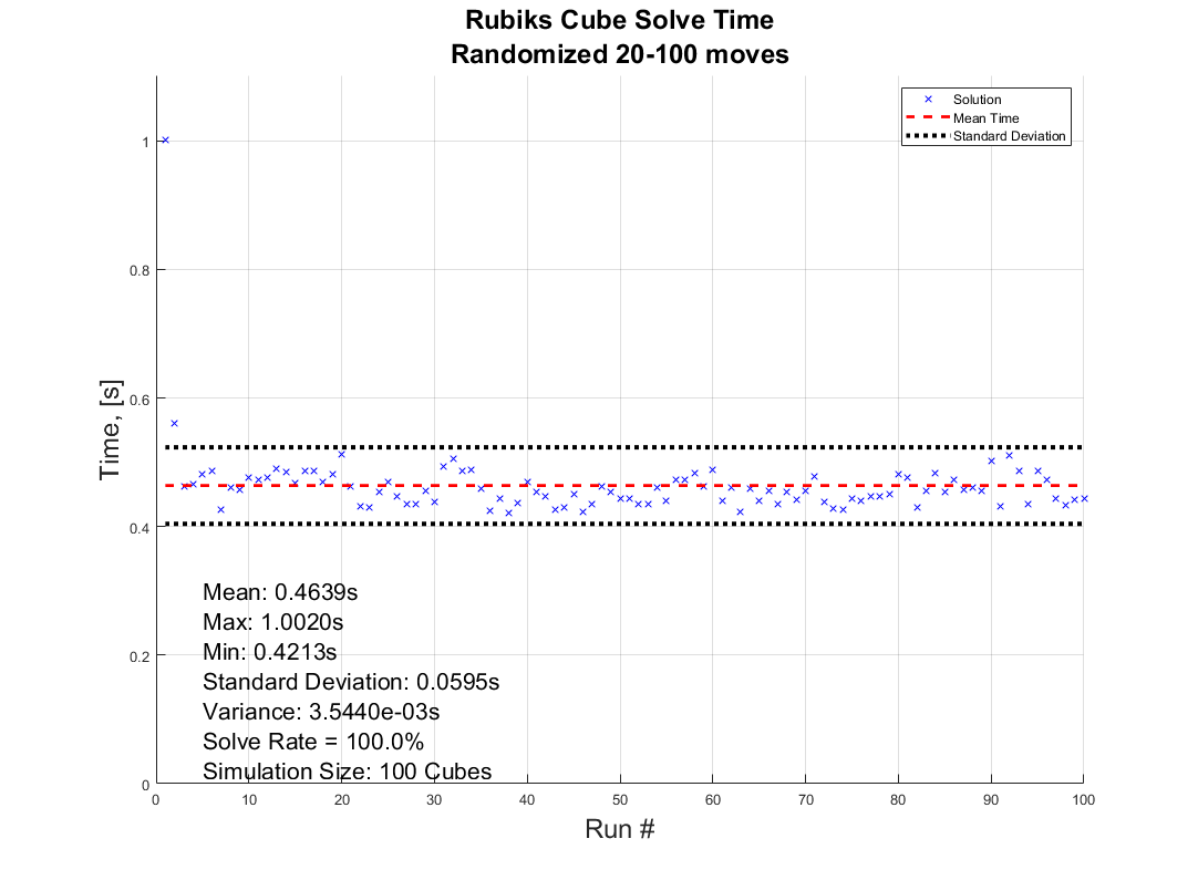
About a year ago, I made a rubix cube solver with the goal of solving a cube faster than I could in real life. It was a fun and educating project, and while it is a long way from optimal, I finished with satisfying results.
How the solver is made is a story for another time, but I always wanted to have a 3D illustration of how the moves are performed to reach the solved state. Lacking the motivation at the time, the illustrative part was forgotten... Untill a couple of weeks ago when I found out about the MATLAB Shorts Mini Hack. It was the perfect motivation to finish up!
This post will detail my entry and remixes (you should check them out before reading!) in this years mini hack. I am not a man to spare any detail, and I've recently saved up a bunch of characters from being limited to 2000, so it may be a bit wordy, but I'll try to keep it entertaining. How it works, lessons learned, sidetracks, pitfalls found, and everything in between is detailed here. So feel free to peruse the sections and pick the ones that sound interesting!
How can I make it move?
Intuativly one would use standard rubix notation to determine the moves, but due to the character limitation and me wanting the ability to rotate the middle rows and the cube as a whole I decided against this.
At the tippy top, there is an 3xn character array, MS, containing the movement sequence of the cube. The three rows contains:
- The axis to rotate around. - Defined by character x, y, z, or p (none of them).
- The row to rotate. - Defined by character 1, 2, 3, or 4 (all of them)
- The direction of the rotation. - Defined by character n, or p (negative or positive)
The rows are ordered from largest to smallest coordinate value along the axis of rotation. If a pause is selected, the program does not really care which character is chosen for the row and direction.
"But how many moves can I make within the time?" As many, or few, as you want.
Well... As long as you want 96 or less moves that is. The function alters the angular speed of the rotations to fit them all within the 96 frame window. But since we iterate through the cube (more on that later) we need to ensure that a move has completely finished before starting another move, or the cube will start looking like a contortionist.
If there is remaining time before the 96 frames are up (due to the timing of the angular speed), the cube politely pauses and waits for the last coule of frames to pass.
The hardest part is finding a sequence short enough to not look like the cube is flailing wildly during its 4 seconds of fame, but long enough to make some interesting pattern like the tetris shuffle in my original entry! Preferably while still being a perfect loop.
I would go on about good seamless loop mechanics, but Vasilis Bellos already made the great post "Creating seamless loop animations by zooming in" last week so I'll just sum it up to make sure to end right before the place you start.
Easy, right? Now go make your own!
Tip: Use the camera rotation to your advantage! Wanting to showcase all sides of the Mathworks cube for as long as possible, I needed a short movement sequence which gives lower angular speed. I cut out two moves from the sequence by making the camera rotate 180 degrees to finish my perfect loop at a different set of coordinates from where I started!
How did you make the cube so beautiful (MathWorks motive)?
A lot of credit should go to Tomoaki Takagi and his entry. I am a sucker for utilizing things for purposes they were not intended to be used for, and he did just that.
We are not allowed to upload images or data in the contest. But we are allowed to optionally upload some background audio for the video. The key is to realise that this audio is stored in the same place as the contest entry. Meaning we can access the "audio.wav" file we just uploaded to the contest.
An audio file is really just a long row of values between -1 and 1. So... if one were to take a picture of every side of a MathWorks cube laying around on the desk, splice the images into 54 seperate textures, scale the intensities between 0 and 1, reshape them to a row, and save it as an .wav file using the audiowrite() function... One would have a bit too much free time, but also a terrible sounding audio file with image data encoded.
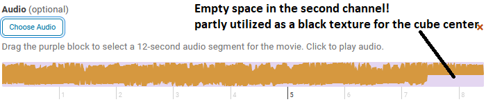
There is one small problem however. As you might have noticed, the audio of most entries sound... rough. This is because of an file compression (or something of the like) applied to files over a certain length when you upload them to the contest. This also applies to audio files filled with image data that does not take particularly well to getting squeezed.
The solution? Compress it yourself (carefully)! Again I looked at Tomoaki's entry, to see what length worked for him. His entry contained a 150x150x3 image upscaled by a factor 4. His image is not exactly sharp, and with 54 different textures needed for a cube, each side would be... about 3x3x3. While a bit poetic, we can not bring such dishonour to such a beautiful object! Luckily Tomoaki had not used the entire audio file for image storage. And he used mono sound (1 audio channel) for his entry and .wav files support stereo sound (2 aoudio channels) meaning I could utilize twice as much space netting me a neat, decent resolution of 28x28 pixels per face!
Don't forget to overwrite the audio on the last frame using audiowrite() however! Most people don't appreciate the sound of images. You should explore Tomoaki's entry for more information on this. The entry is short and easy to understand.
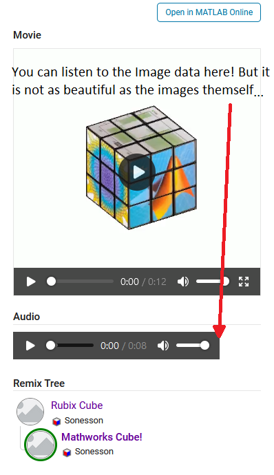
Summary: The audio file uploaded can be used to store image data instead of sound data. Just be careful about file length and size as compression won't treat you kindly!
How did you build the cube?
Excellent question, my dear watsson. Surfaces. Lots and lots of surfaces. This part is takes the most computation time. If anyone has some forbidden knowledge I don't know about here, feel free to correct and enlighten me!
We want to be able to assign each face of the cube a seperate texture, and to be able to move each face seperately without it morphing itself or other parts of the cube. Because of this, they can't be part of a meshgrid connecting each other. Instead we have to construct each surface individually. This takes a second, but is much better in my latest version (See more in the I crave speed section). Which in my earlier entries was a big deal because I was yet to learn about our lord and saviour, persistent variables through Timothy's beautiful entry: Refraction.
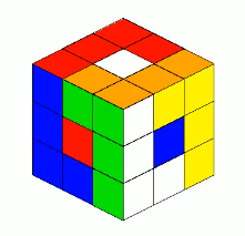
One could think a rubix cube has 54 faces, 9 on each side, but alas that is but an illusion. A rubix cube is infact 27 (26 if not counting the center) smaller cubes in a trench coat. Each with 6 sides. (As illustrated by William Dean's entry Is this cheating? posted while I'm writing this, thanks for the assist!).
Patch objects are all good and well when creating faces if you only want colors, which is the case in my first submission. But MATLAB surface objects are also 3D and have a property that allows them to be textured which we use in the later versions.
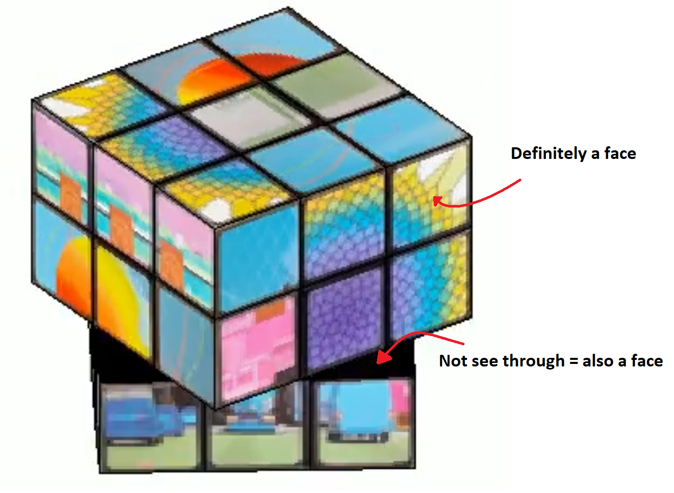
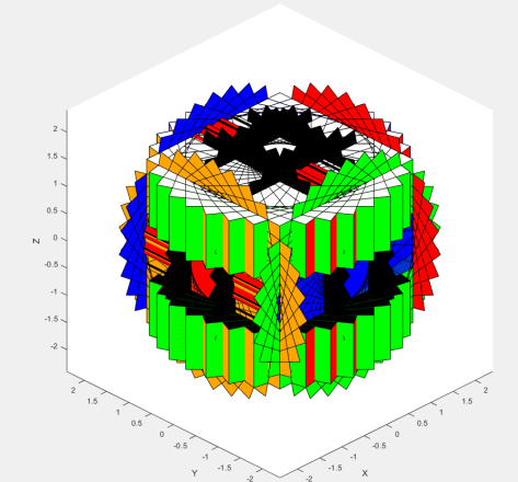
Thinking about the trench coat covered cubes, we can tell that on a physical cube we have 6 planes in each coordinate direction. 2 for each row of cubes. The faces pointing outward are textured and the faces pointing inward are typically black. That is how we will model our cube as well.
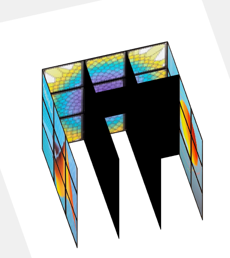
The above image shows how the cube looks during the process of building each face. You may think to yourself "Why do you only have 4 planes in a direction? Do we really need all 6 that you mentioned?" Yes. and if you could enhance and zoom the image like the movies, you would see a tiny gap between the "2" black central planes (this is a surprise tool that will help us later!). The 6 planes are necessary to cover up the cube's hollow interior from multiple viewing angles so we can not compromise it down to 4. Imagine flippnig the cube in the first image of this section and looking into the cube. If we had 4 planes, we would be able to see through the cube from one of the angles.
Summary: We imagine the cube as 3x3x3 smaller cubes. We build each side, inwards pointing or not. We make each face of these smaller cubes seperately using surface() to avoid morphing behavior and to allow the surfaces to be textured individually.
How does it move?
The trick is all about coordinates. Firstly, to make the cube move we need a couple of things:
- Some indicator of how and what to move (a movement sequence, MS)
- The speed at which it should move
- A way to separate what verticies should and should not move
- An operation to transform the coordinates of said verticies so they move
- And of course we need to update the existing data and plot.
We are already familliar with the movement sequence from the first section, so I will spare you the repetition.
The speed of rotation is fairly simple, we have a number of moves defined in MS, and a number of frames to play with, 96. Simply find how many frames we can afford to allocate each move, 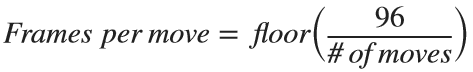 and since each "rotation" of the cube is a quarter turn (
 ) we get
  . Pretty straight forward.
) we get . Pretty straight forward.Now we need to know which verticies should and should not move. Here we use our surprise tool from the previous section! When building the cube, we add a slight offset separating the central planes. We can use this coordinate shift to separate the different planes from eachother. This would not be entierly possible if the central planes shared coordinates.
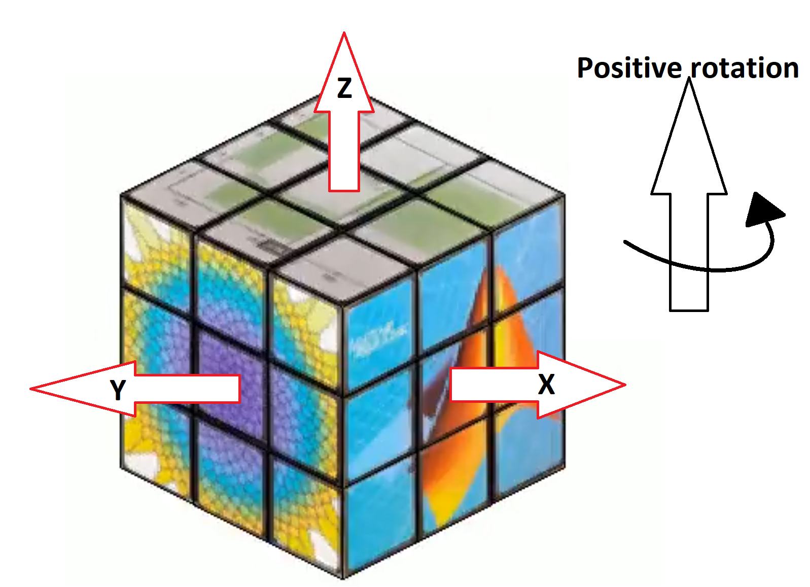
As an example, let's say the movement sequence dictates that we should rotate around x and we should choose the first row. Since the cube is centered around 0 and the planes have coordinates:
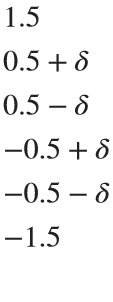
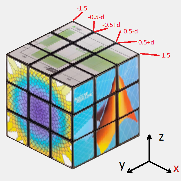
in all directions where δ is the small offset, we can easily seperate the first row by checking which faces have x coordinates higher than 0.5 in all 4 verticies. Simmilarly we check for 4 verticies in between ±0.5 for the 2nd row and values lower than -0.5 for the 3rd row. For rotating the entire cube, we can just select all faces. This works for all coordinate axis due to the symmetry that occurs when being centered around 0.
Now we need an operation to transform the coordinates of the verticies. We want to rotate some 3D coordinates around a specified coordinate axis. Sounds like the perfect job of a rotational matrix for me. This is why you stay in school kids.
In case someone has never heard of a rotation matrix before, on the assumption that anyone using Matrix Laboratory is probably familliar with matrix math and basic linear algebra I'll keep this short. Basically, there are some standard matrices that will rotate a point [x,y,z] arount the origin of an axis. such that
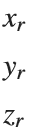 =
= 
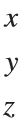
Where the subscripts r denotes the rotated coordinates and ax the axis to rotate around.
These matricies are as follows:
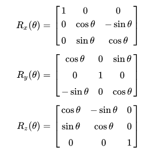
Where θ is the angle with which you rotate the point. In our case the Angular speed.
Now, I define my own rotation matrices. This is because of one of three reasons:
- MATLAB does not have rotation function which rotates a point around a specified axis (this would baffle me)
- I am blind and could not see the correct function in the documentation (plausible)
- I am illiterate and can not read the documentation (improbable)
So we have everything we need! We just update the coordinate data of the affected surface objects, slap down a drawnow command for good measure, and call it an iteration!
But I'd like to shine light on something that is both feature and flaw before we move on. 24 frames per second looks decent enough, but trained eyes can tell it is a bit choppy. Especially when things move fast. So we would like our movement as slow as possible. "Then why does the angular speed as defined above not always utilize all 96 frames to finish the movement sequence?" Because to a trained eye, what looks even more choppy is a rotation not finishing before another starts as the image shows below with a frame by frame on this effect.
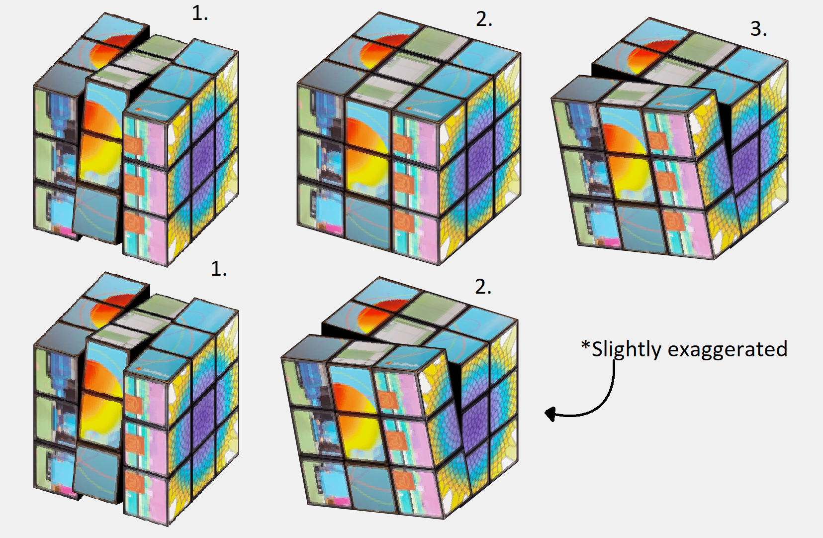
By matching the angular speed to an integer number of frames (by using floor()) for each rotation, we will always complete the entire rotation before starting the next move.This is good because of the reason mentioned above (it looks better), but also because we will base the next rotation on the coordinates of the current position. So it also saves us having to do some extra math to get everything aligned and in position to select the correct faces every time we swap move.
Summary: We use a combination between clever choice of coordinates and some standard rotational matricies to shift the relevant verticies as dictated by the movement sequence by an angle. Being carefull to make each rotation precisely end on an integer number of frames so that the same method works next time.
I crave speed!
Well buckle up then bucko! Best part about programming is that the instant after you spend time making something, you learn something that trivialises it. Persistent variables were that for me this project. My 3rd remix is all about making it faster (in the works as we speak)! You know what they say; "Make it work, make it good, make it fast".
My biggest qualm about my earlier versions was the execution speeds. Every call of drawframe, I would have to rebuild all my surface object to make the cube and re-iterate all the movement of the cube up untill the current frame to ensure the rotations of all verticies, and thus faces, are correct.
Defining a variable as persistent allocates it's memory in a way that it is not removed between function calls. Perfect for being limited by 96 calls to the same function that does not accept iterative input.
Without persistent variables, we needed to remake the surfaces each call to drawframe. Worse still; since we dont know the positions of the surfaces in the previous frame, we also had to re-iterate all the movement of the cube. You may ask yourself "why could you not just calculate the surface position based on the frame, angular speed of rotation and previous moves?". While the position of each face is possible to anticipate effectively with a look up table (which would not fit in the character limit but could have been snuck in with the image data), the rotation of each face is a bit more complex to keep track of. Not an issue with plain colors, but a challange when using textured faces.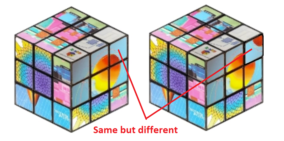
Using persistent variables as in my latest version solves theese two issues and makes the code run silky smooth compared to earlier. It now
- Removes the most time consuming part (creating surfaces) 95 out of 96 times, and
- Removes the need of re-iterating through all movement to catch up with all the rotations previously made.
It does however remove a neat function of the code; frame independency. The competition calls drawframe 96 times with the numbers 1:96, so frame independency it is not an issue as the previous frame is always the previous frame. However, if we now were to call the drawframe function with the values 1, 5 ,and 96, we would not recieve frame number 1, 5, and 96 of the animation as we would have before. Now there is an implicit need to call the function in with the frames in order.
An interesting thought that occured to me was; "If I can store the surface object in a variable, why could i not just copy it to another variable and edit it's properties instead of making a gazillion calls to surface()?" Well, turns out that is not possible because the surface object as stored in the workspace is really more of a pointer to the memory storing the object in the figure window rather than the value in the memory itself. If you copy surface_1 to surface_2 and change surface_2: you get the same change in surface_1.
Also, you might think;
"EWWW... I see nested for loops."
Yep. Is creating the coordinates for the surfaces vectorizable? Absolutely. Not even that hard either. Use combinations() with the possible x, y, and z coordinates and you got yourself the coordinates to every vertice of the cube. Use some fancy logic to determine which vertice goes where and vóila: all verticies neatly ordered ready to be made into surface objects. You could probably even use meshgrid() instead if that is more to your liking. The issue lies in the "made into surface objects" part. As stated, the repeated surface call is still needed to obtain seperate parts of memory to store the surface objects. You would still need as many loop iterations, though not nested. So I decided to leave the nested loops, as a treat, because it made it easier to determine the order and orientations of the textures when encoding them into the audio. After all, efficient coding is not only about the execution speed of the code, it is also about the writing speed of the coder. Or as textbook authors would say: "This is left as an excercise to the reader".
"Are all the inner planes necessary?"
Almost. We need 6 planes for the cube to not look hollow, but since the entire inside plane is black could we not just make it one big surface? No. Different part of the planes move with different rotations, and so can eventually end up as a part of another plane. To avoid morphing, they can not be connected. Also if the planes were solid, we would rotate into still standing planes when a row is angled (kind of like the black parts of the contorted cube earlier). However, we technically do not need the center of the 27 cubes in any scenario, and we could write some logic to not include those specific faces. This was not done for character limitation purposes. I figured that the slight tank in speed would be outweighed by the clean looks and the potential that you, the reader, could achieve when remixing this entry with those sweet sweet roughly 30 extra characters.
"Wait, are you looping... backwards?"
Yes! Looping backwards is a pretty neat trick. In this application it is mainly used to save characters, but runs in roughly the same time as a typical explicit preallocation would.
It works bacause we allocate the first loop value in the last variable element. It is the same principle as writing:
a(5) = 5
As you can see MATLAB will allocate memory for a 5 element vector despite us only specifying one element. So if we start from the back, MATLAB will do the front for us!
And here you can see how it holds up to not preallocating/typical allocation. Plus it gives the same result!
% No preallocation
tic
for i=1:1:10000
x(i) = i;
end
toc
% Typical Preallocation
tic
y=zeros(10000,1);
for i=1:1:10000
y(i) = i;
end
toc
% Backwards looping
tic
for i=10000:-1:1
z(i) = i;
end
toc
% And produces the same results!
all(z==x)
Summary: Persistent variables are really neat They keep their values between calls to functions. In terms of this contest they remove the need to re-iterate things, or for you to keep the state of the last frame without the need for rebuilding it every time.
Surface objects in the workspace are really just pointers to the surface objects in the figure window. This means that we unforttunately must call surface() for each face we want to create.
While initiating the surfaces, I use nested loops. Unnesting these loops is very doable with combination() and left as an excercise to the reader. You will still need the same total number of loop iterations to create all the surface objects, and the loops make texturing more convinient.
All 6 planes are necessary, but the central face of each "inside" plane is redundant and could be skipped at the cost of some additional logic.
Looping backwards is a cool trick to make MATLAB perform the preallocation of memory for you when iterating through a variable.
You get a cube, and you get a cube, and...
As earlier stated, in the "I crave speed!" section my 3 entries happen to follow the "Make it, make it good, make it fast" rule. But I did not just want to upload something that did not add more than just having cleaner code. There is a whole artistic and visual part to it all. So I thought to myself, why not use the speed? Now that the thing is running smooth, why not just run it twice? So i did just that. Except, simmilar results could be achived with much less grief if I just... Made the illusion that I ran it several times in parallel. I wanted to show of the improved speed with making more cubes, but... Why not just copy the cube? So I did that insead!
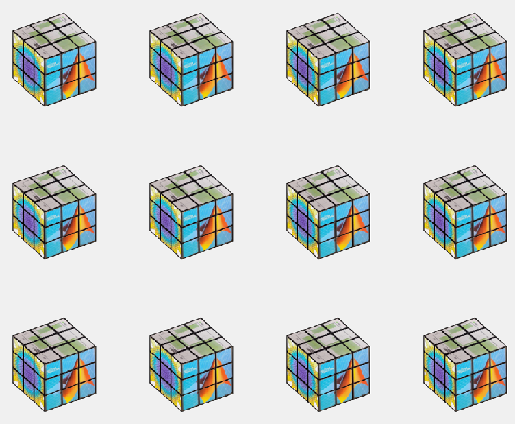
The figure window i really just an interactive image. using getframe()and frame2im() we can quickly turn whatever is shown in the current figure into an image stored in a workspace variable. From here we just need to display that same image multiple times in a sort of array. repmat() in combination with imshow() could have been used here (and would probably have been a bit more flexible in deciding how the cubes are displayed) but I opted for storing the image in a cell array of desired size and using montage() instead.
Most people being character limited in this competition keep everyting to a minimum including the figure windows. Yet I have two of those in my last entry despite only one being shown. As stated in the previous section, surface objects in the workspace is really more of a pointer to the object in the figure, so to keep all my surfaces in between runs I need the figure window containing my surface objects undisturbed. which is why I place the montage in a seperate figure. and display that at the end instead.
An interesting feature *cough* bug *cough* is the swapping between the figure windows that appear in the video generated. This is because of using return as various points in the code in order to skip computations if the move is a 'pause'. The code then does not reach the point where the figure is swaped and montage is made. I thought this to be visually interesting and is therefore dubbing this bug a feature and leaving it in!
Summary:
Multiple cubes were achived by taking the 'image' displayed by the plot window and creating a montage with several of them in a seperate figure window. The swapping between the single and multiple cube view is made by selecting the active figure window before the end of the drawframe call!
Bye for now!
I have yapped on for far too long. Hope you learned something, and thank you all for the kind words and positive response to my entry. This project has been a blast!
T < 2 years
38%
2 years < T < 5 years
26%
5 years < T < 10 years
18%
10 years < T < 20 years
11%
T > 20 years
8%
10172 个投票
Watch episodes 5-7 for the new stuff, but the whole series is really great.
I have one question.
Would it be possible to purchase Matlab for our company and incorporate the functions provided by this software into our in-house developed software to offer it to customers? Is this kind of action permitted under the license terms? I would appreciate advice from someone knowledgeable on this matter.
Inspired by the suggestion of Mr. Chen Lin (MathWorks), I am writing this post with a humble and friendly intent to share some fascinating insights and knowledge about the Schwarzschild radius. My entry, which is related to this post, is named: 'Into the Abyss - Schwarzschild Radius (a time lapse)'.
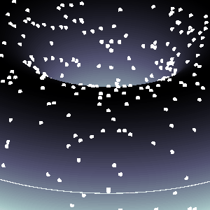
The Schwarzschild radius (or gravitational radius) defines the radius of the event horizon of a black hole, which is the boundary beyond which nothing, not even light, can escape the gravitational pull of the black hole. This concept comes from the Schwarzschild solution to Einstein’s field equations in general relativity. Black holes are regions of spacetime where gravitational collapse has caused matter to be concentrated within such a small volume that the escape velocity exceeds the speed of light.
This is a rudimentary scientific post, as the matter of Schwarzschild radius - it's true meaning and function, is a much, much, much-more complex "thing" (not known to us entierly, by the third degre of epistemological explanation(s)).
And, very important is to mention: I am NOT an expert - by any means, on this topic, just a very curious guy, in almost anything, that has to do with science.
Schwarzschild Radius (Gravitational Radius)
The Schwarzschild radius (Rₛ) is the critical radius at which an object of mass  must be compressed to form a black hole, specifically, a non-rotating, uncharged black hole, known as a Schwarzschild black hole. The Schwarzschild radius
  is given by the formula:
 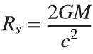 .
.
is given by the formula: . Where: 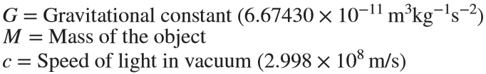 .
.
. Key Characteristics are, that for any mass, if that mass is compressed within a sphere with radius equal to  , the gravitational field is so strong that not even light can escape, thus forming a black hole. The Schwarzschild radius is proportional to the mass. Larger masses have larger Schwarzschild radii.
, the gravitational field is so strong that not even light can escape, thus forming a black hole. The Schwarzschild radius is proportional to the mass. Larger masses have larger Schwarzschild radii.Example:
For the Sun  :
: 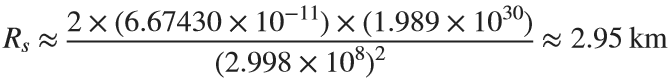 .
.
: .So, if the Sun were compressed into a sphere with a radius of ~3 km, it would become a black hole!
Stellar-mass Black Holes form from the collapse of massive stars (roughly 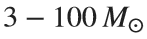 ). Their Schwarzschild radius ranges from a few kilometers to tens of kilometers.
). Their Schwarzschild radius ranges from a few kilometers to tens of kilometers. Supermassive Black Holes found at the centers of galaxies, such as Sagittarius A in the Milky Way ( ), their Schwarzschild radii span from a few million to billions of kilometers!
), their Schwarzschild radii span from a few million to billions of kilometers! Primordial or Micro Black Holes, are the hypothetical small black holes with masses much smaller than stellar masses, where the Schwarzschild radius could be extremely tiny.
A black hole, in general, is a solution to Einstein’s general theory of relativity where spacetime is curved to such an extent that nothing within a certain region, called the event horizon, can escape.
Types of Black Holes:
1. Schwarzschild (Non-rotating, Uncharged):
- This is the simplest type of black hole, described by the Schwarzschild solution.
- Its key feature is the singularity at the center, where the curvature of spacetime becomes infinite.
- No charge, no angular momentum (spin), and spherical symmetry.
2. Kerr (Rotating):
- Describes rotating black holes.
- Involves an additional parameter called angular momentum.
- Has an event horizon and an inner boundary, known as the ergosphere, where spacetime is dragged around by the black hole's rotation.
3. Reissner–Nordström (Charged, Non-rotating):
- A black hole with electric charge.
- A charged black hole has two event horizons (inner and outer) and a central singularity.
4. Kerr–Newman (Rotating and Charged):
- The most general solution, describing a black hole that has both charge and angular momentum.
Relationship Between Schwarzschild Radius and Black Holes
Formation of Black Holes: When a massive star exhausts its nuclear fuel, gravitational collapse can compress the core beyond the Schwarzschild radius, creating a black hole.
Event Horizon: The Schwarzschild radius marks the event horizon for a non-rotating black hole. This is the boundary beyond which no information or matter can escape the black hole.
Curvature of Spacetime: At distances closer than the Schwarzschild radius, spacetime curvature becomes so extreme that all paths, even those of light, are bent towards the black hole’s singularity.
BTW, the term singularity, scientificaly 😊, means that: we do not have a clue what is really happening right there...
Detailed Properties of Black Holes:
a. Singularity:
At the center of a black hole, within the Schwarzschild radius, lies the singularity, a point (or ring in the case of rotating black holes) where gravitational forces compress matter to infinite density and spacetime curvature becomes infinite. General relativity breaks down at the singularity, and a quantum theory of gravity is required for a complete understanding.
b. Event Horizon:
The event horizon is not a physical surface but a boundary where the escape velocity equals the speed of light. For an outside observer, objects falling into a black hole appear to slow down and fade away near the event horizon due to gravitational time dilation, a prediction of general relativity. From the perspective of the infalling object, however, it crosses the event horizon in finite time without noticing anything special at the moment of crossing.
c. Hawking Radiation: (In the post, I told that there is no radiation - to make it simple, although, there is a relatively newly-found (theoretically) radiation. Truth to be said, some physicists are still chalenging this notion, in some of it's parts...)
Quantum mechanical effects near the event horizon predict that black holes can emit radiation (Hawking radiation), a process through which black holes can lose mass and, over very long timescales, potentially evaporate completely. This process has a temperature inversely proportional to the black hole's mass, making large black holes emit extremely weak radiation. (Very trivialy speaking: the concept supposes that an anti-particle is drawn from the vakum and is anihilated with the black's hole matter (particle), and in the process, the black hole looses mass gradually and proportionally to the released energy - very slowly(!)).
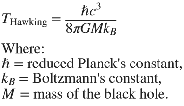
This radiation is significant only for small black holes.
Gravitational Time Dilation (here, as well, things become 'super-weird'...)
Near the Schwarzschild radius, the intense gravitational field leads to time dilation. For an external observer far from the black hole, time appears to slow down for an object moving toward the event horizon. As it approaches the Schwarzschild radius, time dilation becomes so extreme that the object appears frozen in time at the horizon.
The time dilation factor is given by: 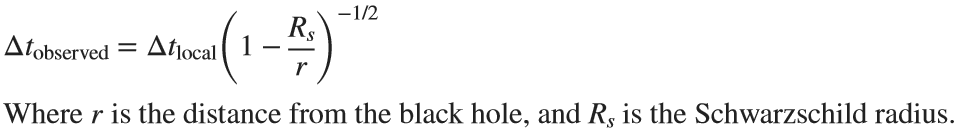
Eg. Approaching the Schwarzschild radius and theoretically remaining just outside of it for a few hours would correspond to the passage of approximately several decades on Earth due to relativistic time dilation.
Using relativistic equations, it's estimated that near the event horizon 2 hours (120 minutes) near the black hole Sagittarius A* (as already mentioned ~ 4 million  ) - in the center of our galaxy Milky Way, could correspond to 83 years passing on Earth! However, this varies based on the precise distance from the event horizon (give or take, a decade 😬).
) - in the center of our galaxy Milky Way, could correspond to 83 years passing on Earth! However, this varies based on the precise distance from the event horizon (give or take, a decade 😬).Information Paradox (definte answer on this question, 'hold's the keys of the universe' 😊, maybe...)
The black hole information paradox arises from the seeming contradiction between general relativity and quantum mechanics.
According to quantum mechanics, information cannot be destroyed, yet anything falling into a black hole seems to be lost beyond the event horizon. Hawking radiation, which allows a black hole to evaporate, does not appear to carry information about the matter that fell into the black hole, leading to ongoing debates and research into how information is preserved in the context of black holes, or not...!
Schwarzschild Radius is the key parameter defining the size of the event horizon of a non-rotating black hole. Black Holes are regions where the Schwarzschild radius constrains all physical phenomena due to extreme gravitational forces, forming event horizons and singularities. The interaction between general relativity and quantum mechanics in the context of black holes (e.g., Hawking radiation and the information paradox) remains one of the most intriguing areas in modern theoretical physics.
For detailed and further reading: https://www.sciencedirect.com/topics/physics-and-astronomy/hawking-radiation.
I hope you will find this post, and information provided, interesting.
This year's MATLAB Shorts Mini Hack contest has kicked off, and there are already lots of interesting entries. The contest features creating a 96-frame, 4-second animation, which is looped 3 times to compose a 12-second short movie. There is an option to add audio to enhance the animation, and it's restricted to a an upper limit of 2,000 characters to promote efficient coding.
Many of the contestants have already realized the potential for creating a seamless loop, which provides a smooth transition and avoids any discontinuities when the animation is repeated. There are several ways to achieve this. An efficient method for example is utilizing sinusoidal functions, which are periodic, meaning that they repeat themselves over time:
An intuitive example of a seamless loop is @Edgar Guevara's EKG pulse entry, which features an electrocardiogram signal on an oscilloscope. The animation is perfectly matched by the audio, as explained in their post.
Another, rather sophisticated approach is featured in @Tim's Moonrun animation in last year's contest. This seamless loop is achieved by cleverly manipulating the camera position and target over a periodic spatial domain, producing this stunning result:
This essentially tells us that for a seamless loop in the spatial domain, the first frame must match the last frame (with a single timestep difference to be more precise, more on that later). But surely this cannot be achieved by zooming in, unless you are simulating a fractal. Well, there are always workarounds.
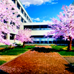
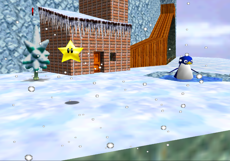
One way to achieve this is by zooming into a section that contains the first frame of the animation. This is featured in my Winter Loop entry. This is a remix of @Oliver Jaros's Winter entry, which was selected as a one of the weekly winners in the nature & space category for Week 1. The code was modified to lower the character count, but all credits for the original idea and graphics go to them. I also drew inspiration from one of my favourite games of all time, Super Mario 64. Oliver's animation reminded me of the Cool, Cool Mountain level of the game. In the game, you can enter various levels by jumping into paintings serving as portals.
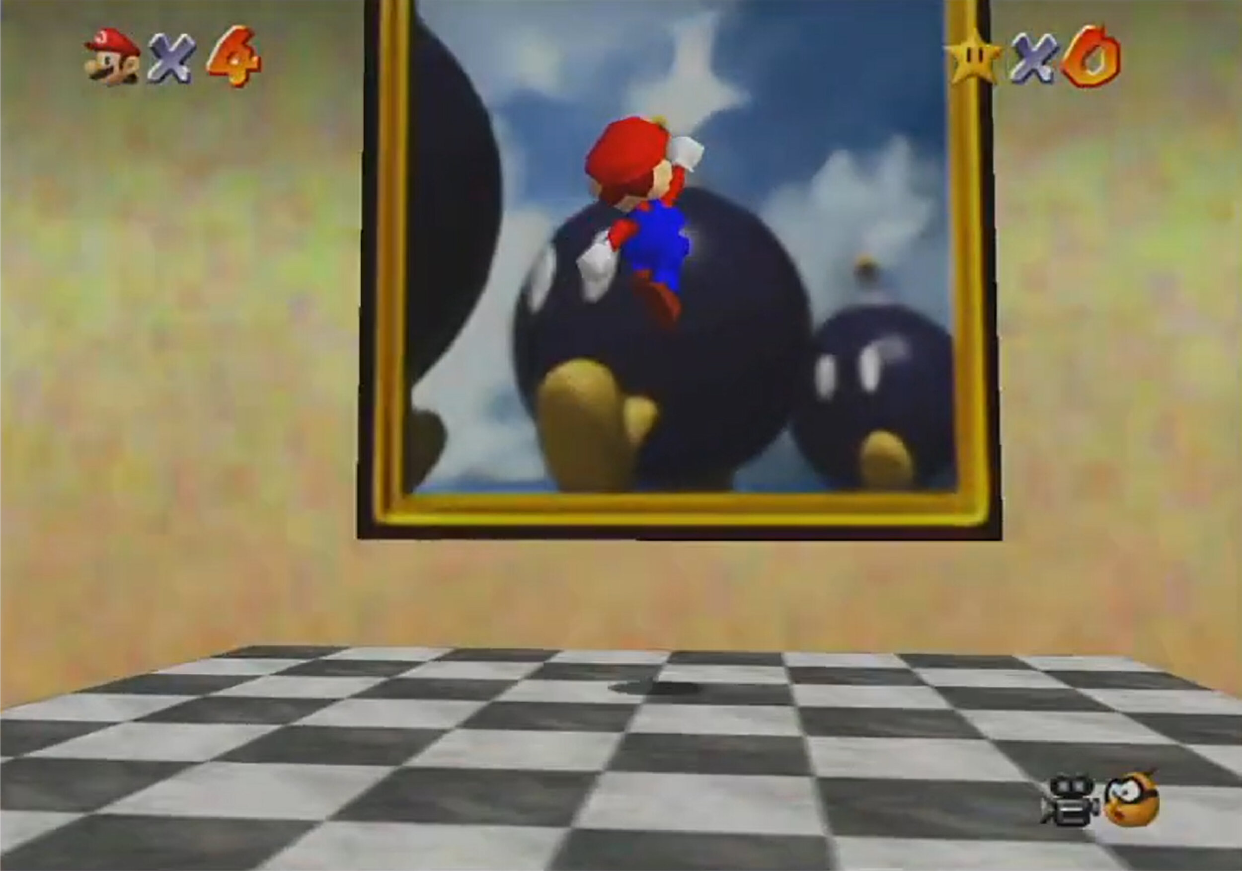
This inspired the idea of zooming into a rectangular photograph frame containing the first frame of the animation to facilitate restarting the loop. One could argue that it would probably take a crazy person to have a photo of their house framed inside their own house. Well, in this economy and with the current house prices, I don't think this scenario is too far-fetched:
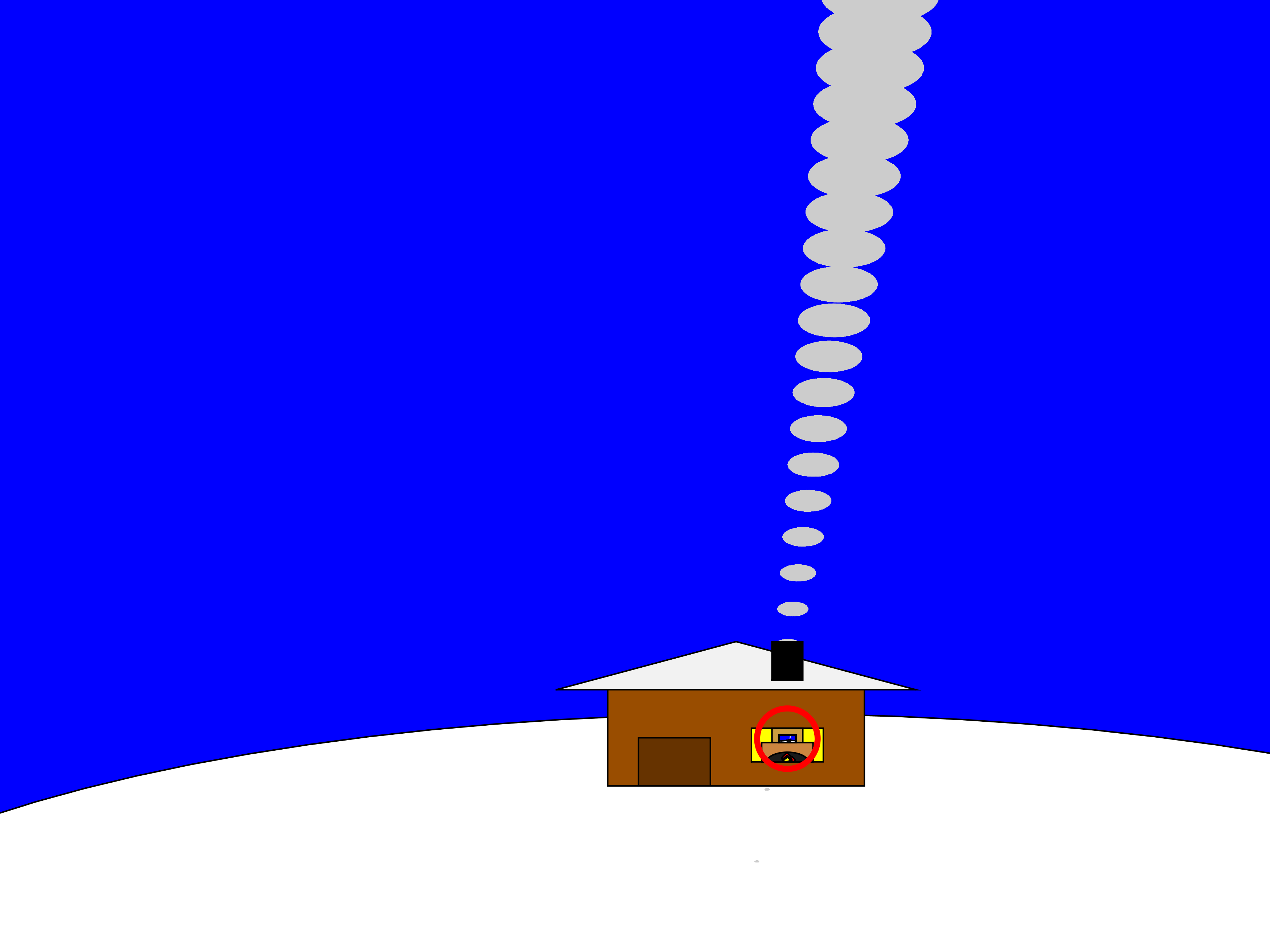
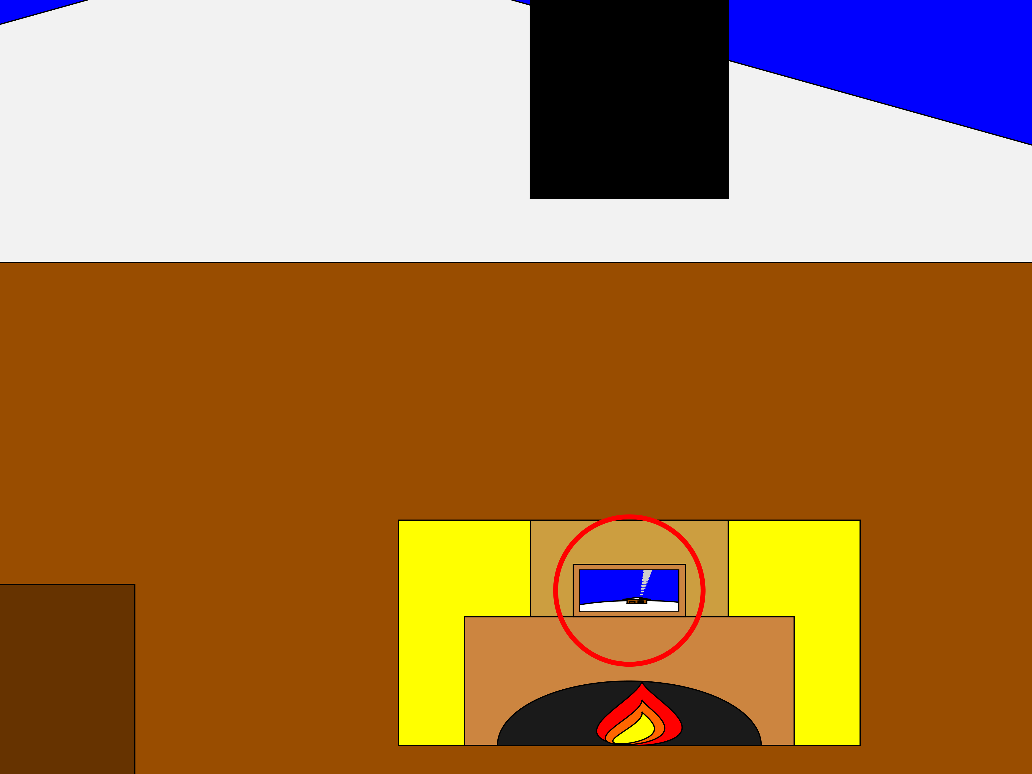
The implementation for this in 2-D is rather simple. Essentially, a second axes is used as the photograph. This is an efficient way of neatly updating the graphics while zooming in. The way this was implemented is explained in the following code snippet, which is a slight modification of the code in the entry:
m = 96; % Number of frames
% Axes limits for the first frame
xm = [xm1,xm2];
ym = [ym1,ym2];
% Axes limits for the last frame (photograph frame edges)
xf = [xf1,xf2];
yf = [yf1,yf2];
% Zoom-in vectors
x1 = linspace(xm(1),xf(1),m+1); % Axes left edge to left photo frame edge
x2 = linspace(xm(2),xf(2),m+1); % Axes right edge to right photo frame edge
y1 = linspace(ym(1),yf(1),m+1); % Axes bottom edge to bottom photo frame edge
y2 = linspace(ym(2),yf(2),m+1); % Axes top edge to top photo frame edge
if f==1
axis([x1(f),x2(f),y1(f),y2(f)]); % Set main axes limits
ax2 = copyobj(gca,gcf); % Create axes for the photo frame containing the first frame graphics objects
end
axis([x1(f+1),x2(f+1),y1(f+1),y2(f+1)]); % Zoom in main axes
lims = axis; % Main axes updated limits
pos = get(gca,'Position'); % Main axes position
% This keeps the relative position of the 2 axes constant:
pos = [pos(1)+diff([lims(1),xf(1)])/diff(lims(1:2))*pos(3),...
pos(2)+diff([lims(3),yf(1)])/diff(lims(3:4))*pos(4),...
diff(xf)/diff(lims(1:2))*pos(3),...
diff(yf)/diff(lims(3:4))*pos(4)];
ax2.Position = pos; % Adjust the relative position
Let's break down the code to explain the process:
- m is the total number of frames in the animation, i.e. 96 frames.
- xm & ym are the main axes limits for frame 1.
- xf & yf are the main axes limits for frame 96, corresponding to the photograph frame's edges.
- x1, x2, y1 & y2 are the zoom-in vectors, linearly spaced from the left, right, bottom & top main axes edges to the corresponding photograph edges. You have probably noticed that these contain m+1=97 points, which is 1 more than the total number of frames. This is done so that the first frame of the animation and the contents of the photograph frame are offset by a single timestep, so that there are no overlapping frames when the animation is looped, thus creating a perfect, seamless loop. That means that the first frame of the animation will contain the main axes zoomed-in by a single timestep, while the last frame of the animation (i.e. the zoomed-in photograph frame) will contain the most zoomed-out version of the graphics. This neatly wraps the animation, and displays the full zoomed-out view when the video stops playing.
- The photograph frame axes are created when f==1 (after setting the initial axes limits) by using the immensely useful copyobj function. This one-liner creates axes containing all graphics objects for the first frame.
- Zooming in on the main axes is then achieved by adjusting the limits using axis([x1(f+1),x2(f+1),y1(f+1),y2(f+1)]). The main axes current limits and position are then saved using the variables lims and pos respectively, in order to adjust the position of the photograph frame axes.
- While zooming in, it's important that the relative position of the 2 axes is kept constant. This is achieved by simply adjusting the position of the photograph frame axes at every frame, by calculating their relative ratios using the abovementioned formula. The first 2 arguments correspond to the (normalized) x and y positions of the lower left corner of the axes, while the third and fourth arguments correspond to the (normalized) width and height respectively. While this formula will work for any position of the main axes, it's a good idea to set the position as set(gca,'Position',[0 0 1 1]) for this contest, in order to take full advantage of the whole allocated window for the animation.
- Finally, note that the graphics are updated for the main axes only, and the above process is repeated for each frame until fully zooming into the photograph frame's axes.
Some of the most curious minds might wonder that while this is well and all with using the second axes to simulate the photograph, what happens to the photograph inside the photograph (and so on...)? Well, the beauty of this method is that you can repeat this as many times as necessary (just apply the formula using the current position and limits of the second axes to adjust the position of the third axes and so on). Given the speed of the animation and the very small size of the photograph inside the photograph, it would be very unlikely that you would need more than 3 axes, but the process is always good to know.
This is the final result:
I hope you found these tips useful and I'm looking forward to seeing many creative seamless loop animations in the contest.
MAThematical LABor
3%
MAth Theory Linear AlgeBra
12.5%
MATrix LABoratory
84%
MATthew LAst Breakthrough
0%
32 个投票
At School / university
64%
At work
30%
At home
3%
Elsewhere
3%
33 个投票
I am using Mathlab/simulink R2023b and PSIM2022.1.
I am trying to do co-simulación betwen simulink and PSIM of multiport controlled inverters. In Simulink, when I add the simcoupler block and double clik in it to set the path, that windows is opened, but when browse the path of PSIM schematic file and then clik APPLY, suddenly Simulink closes. Could somebody give some clue How to solve this issue.
NOTE: I tried as well the example of the tutorial of simcoupler module but the problem is the same.
您也可以从以下列表中选择网站:
美洲
- América Latina (Español)
- Canada (English)
- United States (English)
欧洲
- Belgium (English)
- Denmark (English)
- Deutschland (Deutsch)
- España (Español)
- Finland (English)
- France (Français)
- Ireland (English)
- Italia (Italiano)
- Luxembourg (English)
- Netherlands (English)
- Norway (English)
- Österreich (Deutsch)
- Portugal (English)
- Sweden (English)
- Switzerland
- United Kingdom(English)
亚太
- Australia (English)
- India (English)
- New Zealand (English)
- 中国
- 日本Japanese (日本語)
- 한국Korean (한국어)