主要内容
Results for
Can you solve it?
This study explores the demographic patterns and disease outcomes during the cholera outbreak in London in 1849. Utilizing historical records and scholarly accounts, the research investigates the impact of the outbreak on the city' s population. While specific data for the 1849 cholera outbreak is limited, trends from similar 19th - century outbreaks suggest a high infection rate, potentially ranging from 30% to 50% of the population, owing to poor sanitation and overcrowded living conditions . Additionally, the birth rate in London during this period was estimated at 0.037 births per person per year . Although the exact reproduction number (R₀) for cholera in 1849 remains elusive, historical evidence implies a high R₀ due to the prevalent unsanitary conditions . This study sheds light on the challenges of estimating disease parameters from historical data, emphasizing the critical role of sanitation and public health measures in mitigating the impact of infectious diseases.
Introduction
The cholera outbreak of 1849 was a significant event in the history of cholera, a deadly waterborne disease caused by the bacterium Vibrio cholera. Cholera had several major outbreaks during the 19th century, and the one in 1849 was particularly devastating.
During this outbreak, cholera spread rapidly across Europe, including countries like England, France, and Germany . The disease also affected North America, with outbreaks reported in cities like New York and Montreal. The exact number of casualties from the 1849 cholera outbreak is difficult to determine due to limited record - keeping at that time. However, it is estimated that tens of thousands of people died as a result of the disease during this outbreak.
Cholera is highly contagious and spreads through contaminated water and food . The lack of proper sanitation and hygiene practices in the 19th century contributed to the rapid spread of the disease. It wasn't until the late 19th and early 20th centuries that advancements in public health, sanitation, and clean drinking water significantly reduced the incidence and impact of cholera outbreaks in many parts of the world.
Infection Rate
Based on general patterns observed in 19th - century cholera outbreaks and the conditions of that time, it' s reasonable to assume that the infection rate was quite high. During major cholera outbreaks in densely populated and unsanitary areas, infection rates could be as high as 30 - 50% or even more.
This means that in a densely populated city like London, with an estimated population of around 2.3 million in 1849, tens of thousands of people could have been infected during the outbreak. It' s important to emphasize that this is a rough estimation based on historical patterns and not specific to the 1849 outbreak. The actual infection rate could have varied widely based on the local conditions, public health measures in place, and the effectiveness of efforts to contain the disease.
For precise and localized estimations, detailed historical records specific to the 1849 cholera outbreak in a particular city or region would be required, and such data might not be readily available due to the limitations of historical documentation from that time period
Mortality Rate
It' s challenging to provide an exact death rate for the 1849 cholera outbreak because of the limited and often unreliable historical records from that time period. However, it is widely acknowledged that the death rate was significant, with tens of thousands of people dying as a result of the disease during this outbreak.
Cholera has historically been known for its high mortality rate, particularly in areas with poor sanitation and limited access to clean water. During cholera outbreaks in the 19th century, mortality rates could be extremely high, sometimes reaching 50% or more in affected communities. This high mortality rate was due to the rapid onset of severe dehydration and electrolyte imbalance caused by the cholera toxin, leading to death if not promptly treated.
Studies and historical accounts from various cholera outbreaks suggest that the R₀ for cholera can range from 1.5 to 2.5 or even higher in conditions where sanitation is inadequate and clean water is scarce. This means that one person with cholera could potentially infect 1.5 to 2.5 or more other people in such settings.
Unfortunately, there are no specific and reliable data available regarding the recovery rates from the 1849 cholera outbreak, as detailed and accurate record - keeping during that time period was limited. Cholera outbreaks in the 19th century were often devastating due to the lack of effective medical treatments and poor sanitation conditions. Recovery from cholera largely depended on the individual's ability to rehydrate, which was difficult given the rapid loss of fluids through severe diarrhea and vomiting .
LONDON CASE OF STUDY
In 1849, the estimated population of London was around 2.3 million people. London experienced significant population growth during the 19th century due to urbanization and industrialization. It’s important to note that historical population figures are often estimates, as comprehensive and accurate record-keeping methods were not as advanced as they are today.
% Define parameters
R0 = 2.5;
beta = 0.5;
gamma = 0.2; % Recovery rate
N = 2300000; % Total population
I0 = 1; % Initial number of infected individuals
% Define the SIR model differential equations
sir_eqns = @(t, Y) [-beta * Y(1) * Y(2) / N; % dS/dt
beta * Y(1) * Y(2) / N - gamma * Y(2); % dI/dt
gamma * Y(2)]; % dR/dt
% Initial conditions
Y0 = [N - I0; I0; 0]; % Initial conditions for S, I, R
% Time span
tmax1 = 100; % Define the maximum time (adjust as needed)
tspan = [0 tmax1];
% Solve the SIR model differential equations
[t, Y] = ode45(sir_eqns, tspan, Y0);
% Plot the results
figure;
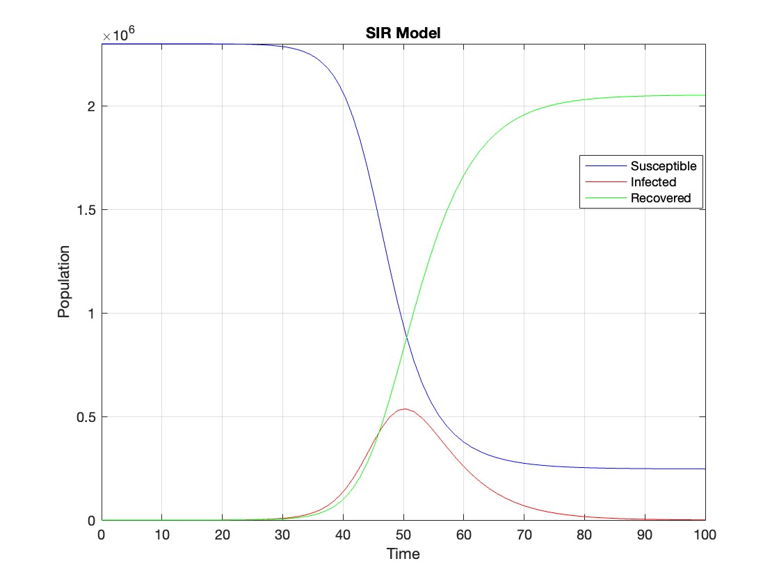
plot(t, Y(:,1), 'b', t, Y(:,2), 'r', t, Y(:,3), 'g');
legend('Susceptible', 'Infected', 'Recovered');
xlabel('Time');
ylabel('Population');
title('SIR Model');
axis tight;
grid on;
% Assuming t and Y are obtained from the ode45 solver for the SIR model
% Extract the infected population data (second column of Y)
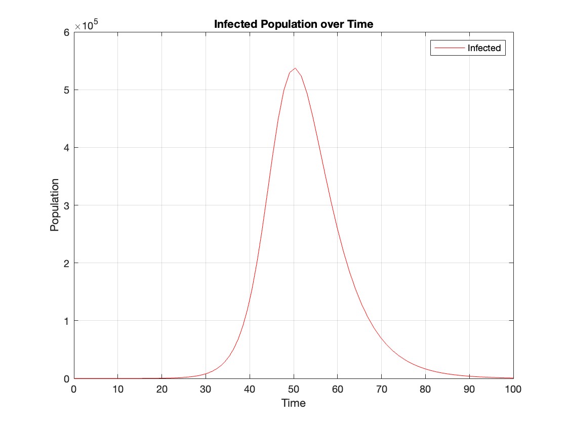
infected = Y(:,2);
% Plot the infected population over time
figure;
plot(t, infected, 'r');
legend('Infected');
xlabel('Time');
ylabel('Population');
title('Infected Population over Time');
grid on;
The code provides a visual representation of how the disease spreads and eventually diminishes within the population over the specified time interval . It can be used to understand the impact of different parameters (such as infection and recovery rates) on the progression of the outbreak .
The study of nonlinear dynamical systems in lattices is an area of research with continuously growing interest.The first systematic studies of these systems emerged in the late 1930 s,thanks to the work of Frenkel and Kontorova on crystal dislocations.These studies led to the formulation of the discrete Klein-Gordon equation (DKG).Specifically,in 1939,Frenkel and Kontorova proposed a model that describes the structure and dynamics of a crystal lattice in a dislocation core.The FK model has become one of the fundamental models in physics,as it has been proven to reliably describe significant phenomena observed in discrete media.The equation we will examine is a variation of the following form:

The process described involves approximating a nonlinear differential equation through the Taylor method and simplifying it into a linear model.Let's analyze step by step the process from the initial equation to its final form.For small angles, can be approximated through the Taylor series as:
We substitute  in the original equation with the Taylor approximation:
To map this equation to a linear model,we consider the angles  to correspond to displacements
  in a mass-spring system.Thus,the equation transforms into:
to correspond to displacements We recognize that the term  expresses the nonlinearity of the system,while β is a coefficient corresponding to this nonlinearity,simplifying the expression.The final form of the equation is:
The exact value of β depends on the mapping of coefficients in the Taylor approximation and its application to the specific physical problem.Our main goal is to derive results regarding stability and convergence in nonlinear lattices under nonlinear conditions.We will examine the basic characteristics of the discrete Klein-Gordon equation:
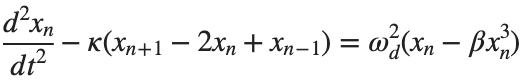
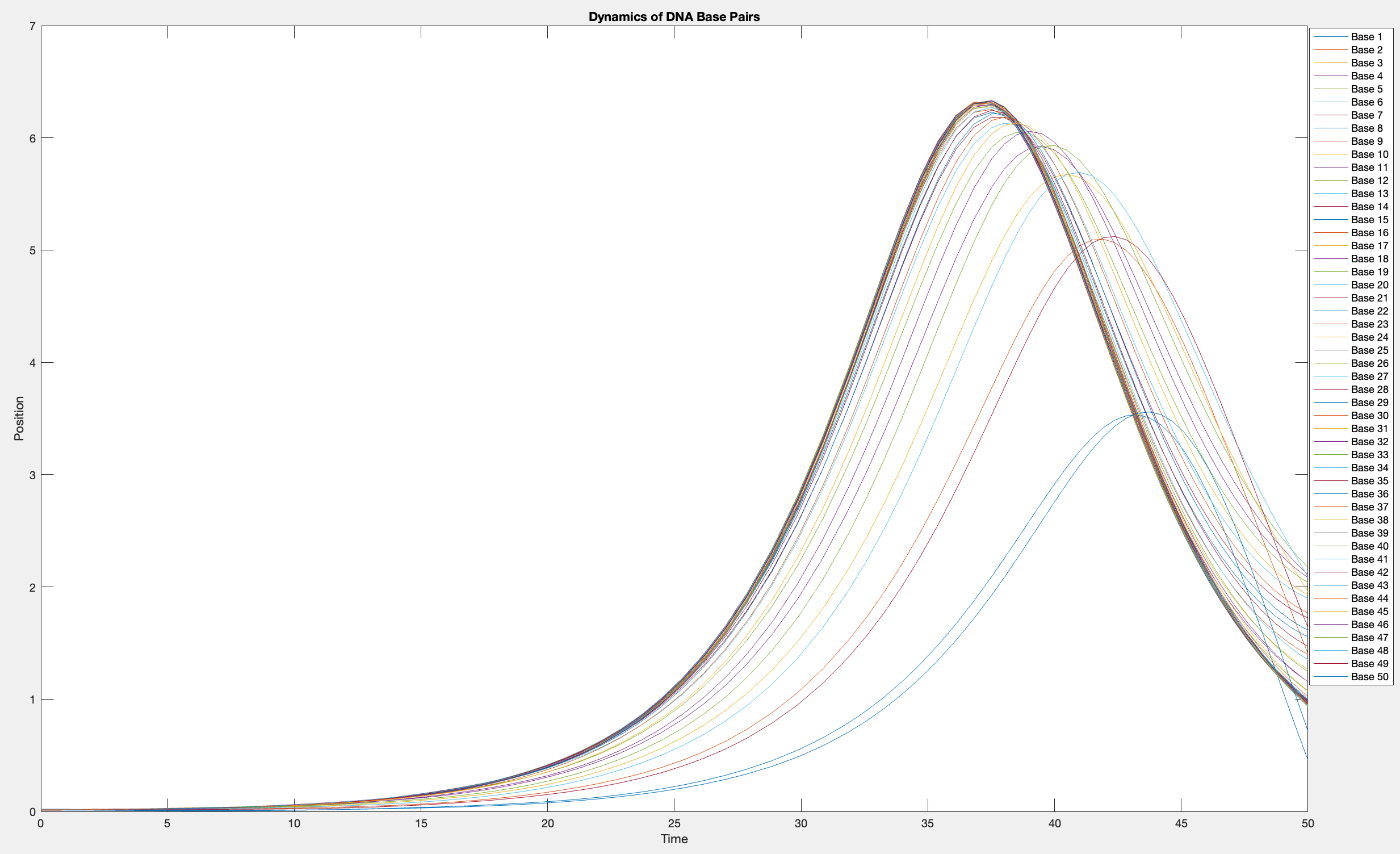
This model is often used to describe the opening of the DNA double helix during processes such as transcription.The model focuses on the transverse motion of the base pairs,which can be represented by a set of coupled nonlinear differential equations.
% Parameters
numBases = 50; % Number of base pairs
kappa = 0.1; % Elasticity constant
omegaD = 0.2; % Frequency term
beta = 0.05; % Nonlinearity coefficient
% Initial conditions
initialPositions = 0.01 + (0.02 - 0.01) * rand(numBases, 1);
initialVelocities = zeros(numBases, 1);
Time span
tSpan = [0 50];
>> % Differential equations
odeFunc = @(t, y) [y(numBases+1:end); ... % velocities
kappa * ([y(2); y(3:numBases); 0] - 2 * y(1:numBases) + [0; y(1:numBases-1)]) + ...
omegaD^2 * (y(1:numBases) - beta * y(1:numBases).^3)]; % accelerations
% Solve the system
[T, Y] = ode45(odeFunc, tSpan, [initialPositions; initialVelocities]);
% Visualization
plot(T, Y(:, 1:numBases))
legend(arrayfun(@(n) sprintf('Base %d', n), 1:numBases, 'UniformOutput', false))
xlabel('Time')
ylabel('Position')
title('Dynamics of DNA Base Pairs')
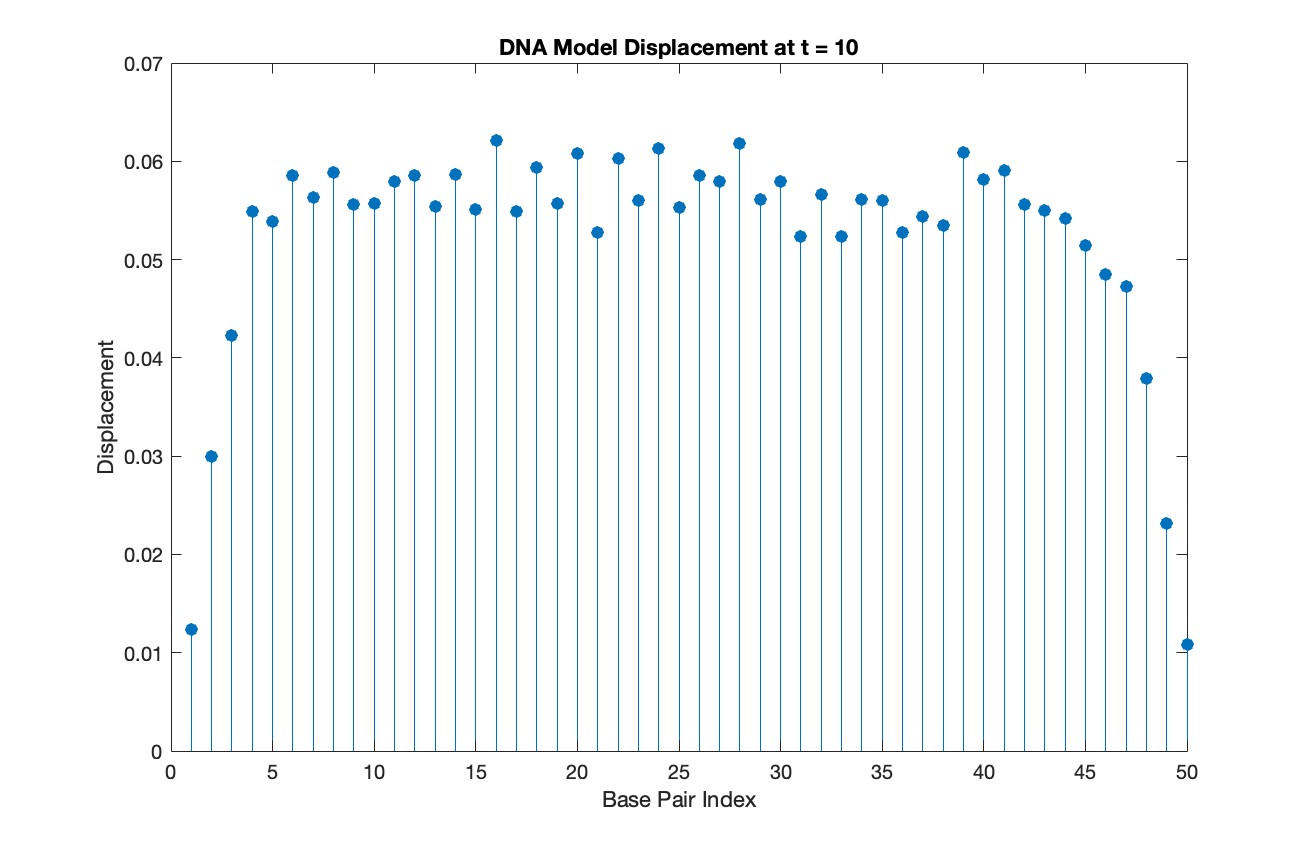
% Choose a specific time for the snapshot
snapshotTime = 10;
% Find the index in T that is closest to the snapshot time
[~, snapshotIndex] = min(abs(T - snapshotTime));
% Extract the solution at the snapshot time
snapshotSolution = Y(snapshotIndex, 1:numBases);
% Generate discrete plot for the DNA model at the snapshot time
figure;
stem(1:numBases, snapshotSolution, 'filled')
title(sprintf('DNA Model Displacement at t = %d', snapshotTime))
xlabel('Base Pair Index')
ylabel('Displacement')
% Time vector for detailed sampling
tDetailed = 0:0.5:50;
% Initialize an empty array to hold the data
data = [];
% Generate the data for 3D plotting
for i = 1:numBases
% Interpolate to get detailed solution data for each base pair
detailedSolution = interp1(T, Y(:, i), tDetailed);
% Concatenate the current base pair's data to the main data array
data = [data; repmat(i, length(tDetailed), 1), tDetailed', detailedSolution'];
end
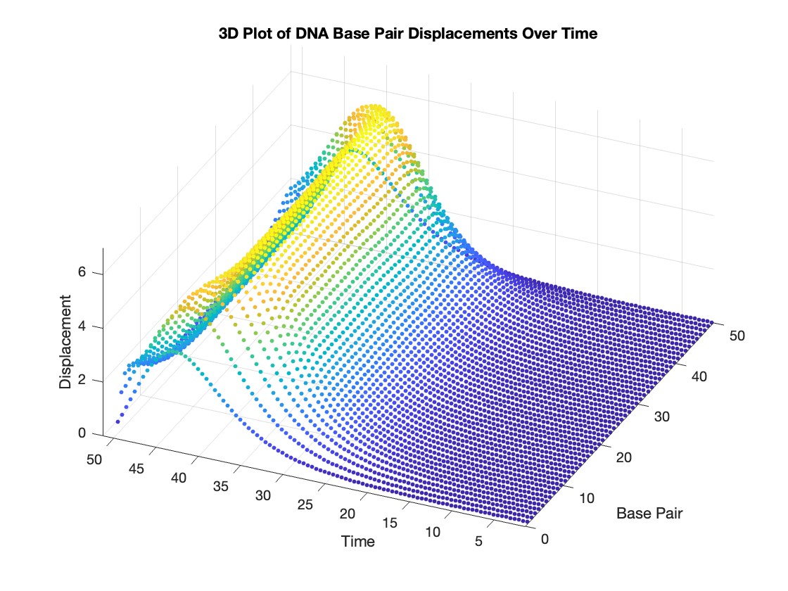
% 3D Plot
figure;
scatter3(data(:,1), data(:,2), data(:,3), 10, data(:,3), 'filled')
xlabel('Base Pair')
ylabel('Time')
zlabel('Displacement')
title('3D Plot of DNA Base Pair Displacements Over Time')
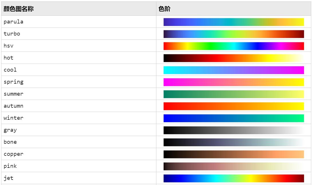
colormap('rainbow')
colorbar
Lots of students like me have a break from school this week or next! If y'all are looking for something interesting to do learn a bit about using hgtransform by making the transforming snake animation in MATLAB!
Code below!
⬇️⬇️⬇️
numblock=24;
v = [ -1 -1 -1 ; 1 -1 -1 ; -1 1 -1 ; -1 1 1 ; -1 -1 1 ; 1 -1 1 ];
f = [ 1 2 3 nan; 5 6 4 nan; 1 2 6 5; 1 5 4 3; 3 4 6 2 ];
clr = hsv(numblock);
shapes = [ 1 0 0 0 0 0 1 0 0 0 0 1 0 0 0 0 0 0 1 0 0 0 0 1 % box
0 0 .5 -.5 .5 0 1 0 -.5 .5 -.5 0 1 0 .5 -.5 .5 0 1 0 -.5 .5 -.5 0 % fluer
0 0 1 1 0 .5 -.5 1 .5 .5 -.5 -.5 1 .5 .5 -.5 -.5 1 .5 .5 -.5 -.5 1 .5 % bowl
0 .5 -.5 -.5 .5 -.5 .5 .5 -.5 .5 -.5 -.5 .5 -.5 .5 .5 -.5 .5 -.5 -.5 .5 -.5 .5 .5]; % ball
% Build the assembly
set(gcf,'color','black');
daspect(newplot,[1 1 1]);
xform=@(R)makehgtform('axisrotate',[0 1 0],R,'zrotate',pi/2,'yrotate',pi,'translate',[2 0 0]);
P=hgtransform('Parent',gca,'Matrix',makehgtform('xrotate',pi*.5,'zrotate',pi*-.8));
for i = 1:numblock
P = hgtransform('Parent',P,'Matrix',xform(shapes(end,i)*pi));
patch('Parent',P, 'Vertices', v, 'Faces', f, 'FaceColor',clr(i,:),'EdgeColor','none');
patch('Parent',P, 'Vertices', v*.75, 'Faces', f(end,:), 'FaceColor','none',...
'EdgeColor','w','LineWidth',2);
end
view([10 60]);
axis tight vis3d off
camlight
% Setup vectors for animation
h=findobj(gca,'type','hgtransform')'; h=h(2:end);
r=shapes(end,:)*pi;
steps=100;
% Animate between different shapes
for si = 1:size(shapes,1)
sh = shapes(si,:)*pi;
diff = (sh-r)/steps;
% Animate to a new shape
for s=1:steps
arrayfun(@(tx)set(h(tx),'Matrix',xform(r(tx)+diff(tx)*s)),1:numblock);
view([s*360/steps 20]); drawnow();
end
r=sh;
for s=1:steps; view([s*360/steps 20]); drawnow(); end % finish rotate
end
Chord diagrams are very common in Python and R, but there are no related functions in MATLAB before. It is not easy to draw chord diagrams of the same quality as R language, But I created a MATLAB tool that could almost do it.
↓ ↓ ↓ ↓ ↓ ↓ ↓ ↓ ↓ ↓
↑ ↑ ↑ ↑ ↑ ↑ ↑ ↑ ↑ ↑
Here is the help document:
1 Data Format
The data requirement is a numerical matrix with all values greater than or equal to 0, or a table array, or a numerical matrix and cell array for names. First, give an example of a numerical matrix:
1.1 Numerical Matrix
dataMat=randi([0,5],[5,4]);
% 绘图(draw)
CC=chordChart(dataMat);
CC=CC.draw();
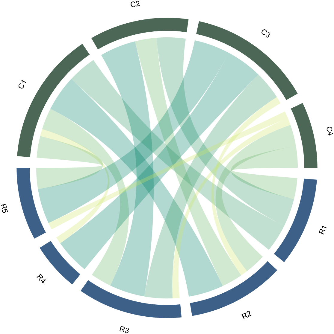
Since each object is not named, it will be automatically named Rn and Cn
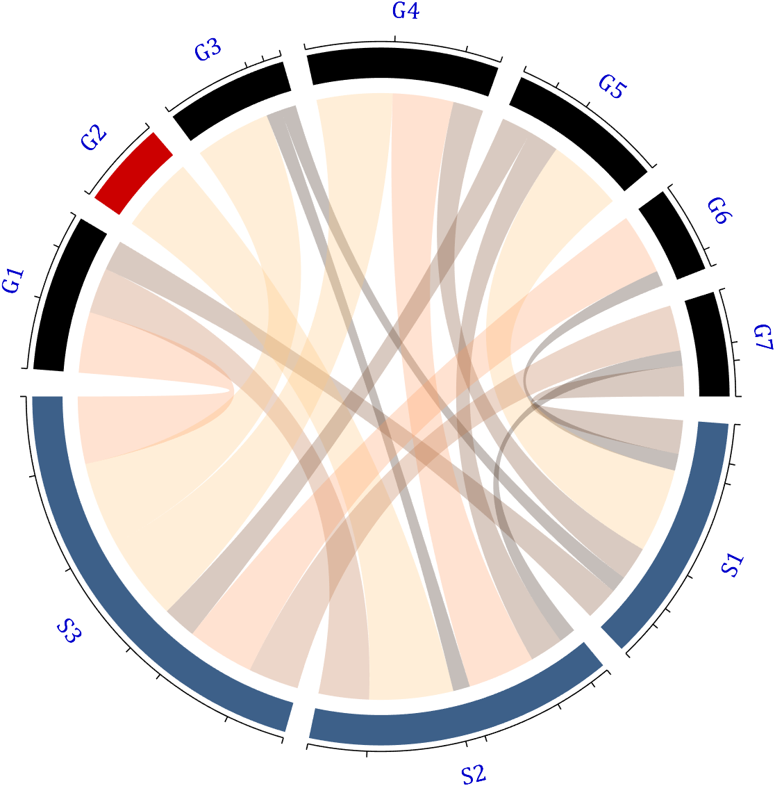
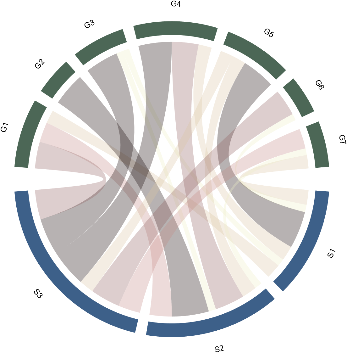
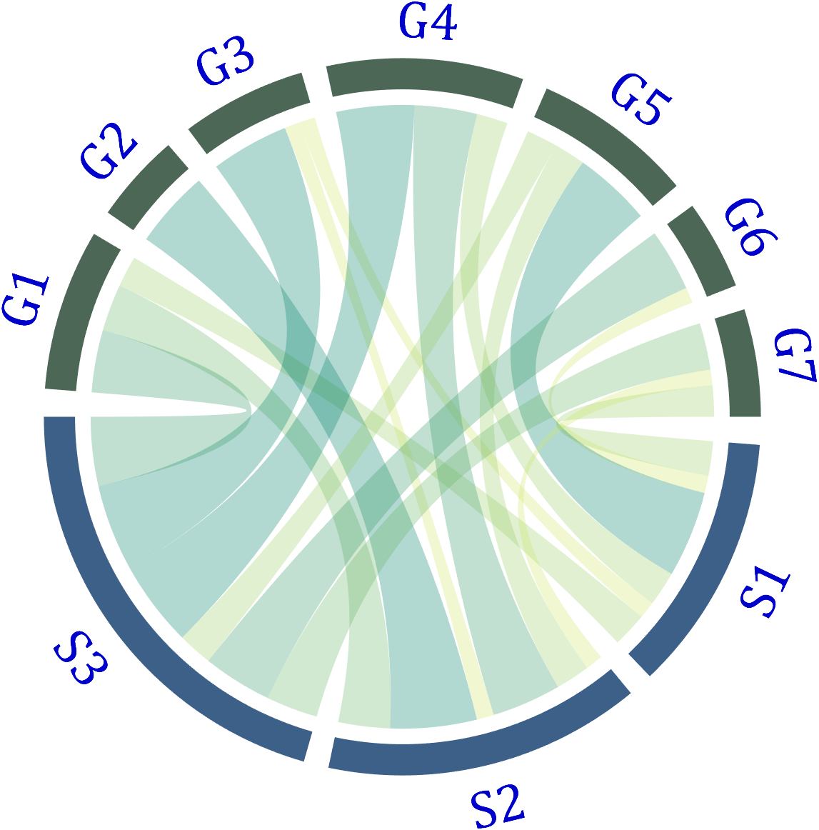
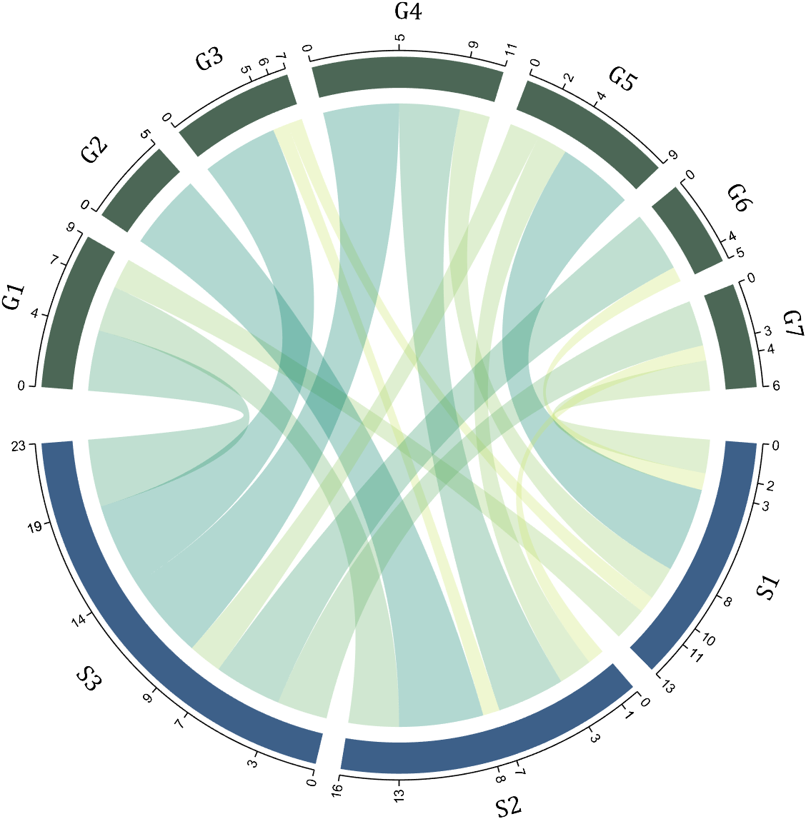
1.2 Numerical Matrix and Cell Array for Names
dataMat=[2 0 1 2 5 1 2;
3 5 1 4 2 0 1;
4 0 5 5 2 4 3];
colName={'G1','G2','G3','G4','G5','G6','G7'};
rowName={'S1','S2','S3'};
CC=chordChart(dataMat,'rowName',rowName,'colName',colName);
CC=CC.draw();

RowName should be the same size as the rows of the matrix
ColName should be the same size as the columns of the matrix
For this example, if the value in the second row and third column is 1, it indicates that there is an energy flow from S2 to G3, and a chord with a width of 1 is needed between these two.
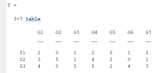
1.3 Table Array
A table array in the following format is required:
2 Decorate Chord
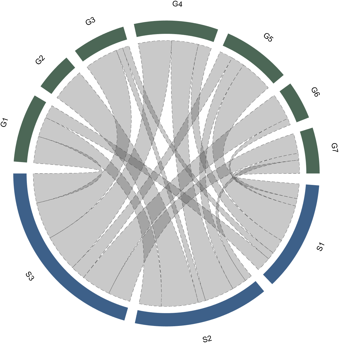
2.1 Batch modification of chords
Batch modification of chords can be done using the setChordProp function, and all properties of the Patch object can be modified. For example, modifying the color of the string, edge color, edge line sstyle, etc.:
CC.setChordProp('EdgeColor',[.3,.3,.3],'LineStyle','--',...
'LineWidth',.1,'FaceColor',[.3,.3,.3])
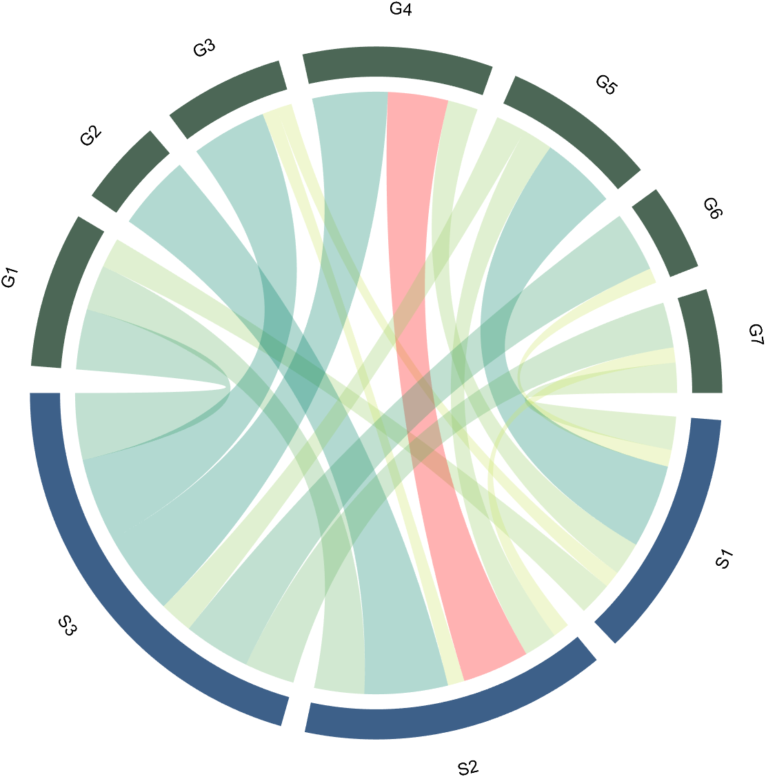
2.2 Individual Modification of Chord
The individual modification of chord can be done using the setChordMN function, where the values of m and n correspond exactly to the rows and columns of the original numerical matrix. For example, changing the color of the strings flowing from S2 to G4 to red:
CC.setChordMN(2,4,'FaceColor',[1,0,0])
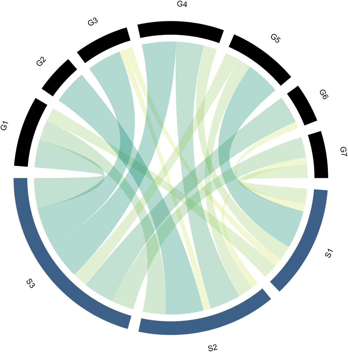
2.3 Color Mapping of Chords
Just use function colormap to do so:
% version 1.7.0更新
% 可使用colormap函数直接修改颜色
% Colors can be adjusted directly using the function colormap(demo4)
colormap(flipud(pink))
3 Arc Shaped Block Decoration
3.1 Batch Decoration of Arc-Shaped Blocks
use:
- setSquareT_Prop
- setSquareF_Prop
to modify the upper and lower blocks separately, and all attributes of the Patch object can be modified. For example, batch modify the upper blocks (change to black):
CC.setSquareT_Prop('FaceColor',[0,0,0])
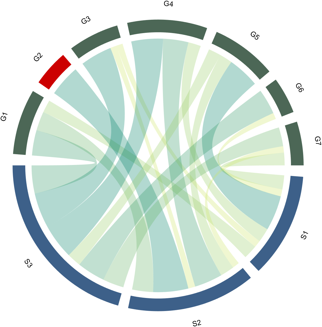
3.2 Arc-Shaped Blocks Individually Decoration
use:
- setSquareT_N
- setSquareF_N
to modify the upper and lower blocks separately. For example, modify the second block above separately (changed to red):
CC.setSquareT_N(2,'FaceColor',[.8,0,0])
4 Font Adjustment
Use the setFont function to adjust the font, and all properties of the text object can be modified. For example, changing the font size, font, and color of the text:
CC.setFont('FontSize',25,'FontName','Cambria','Color',[0,0,.8])
5 Show and Hide Ticks
Usage:
CC.tickState('on')
% CC.tickState('off')
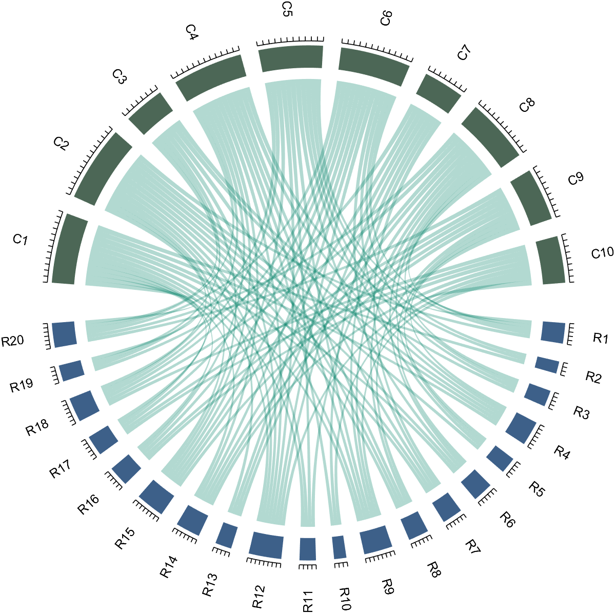
6 Attribute 'Sep' with Adjustable Square Spacing
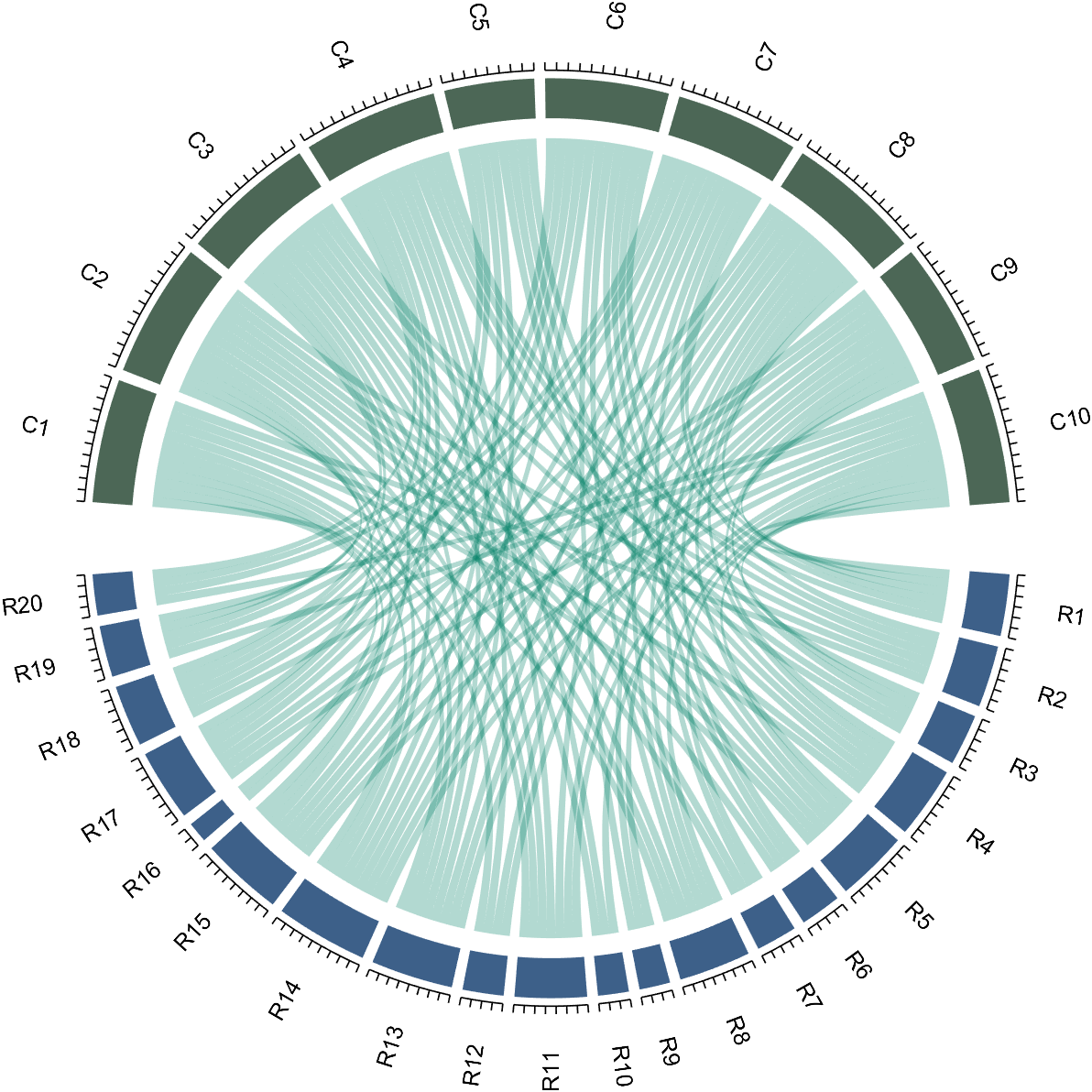
If the matrix size is large, the drawing will be out of scale:
dataMat=randi([0,1],[20,10]);
CC=chordChart(dataMat);
CC=CC.draw();
% CC.tickState('on')
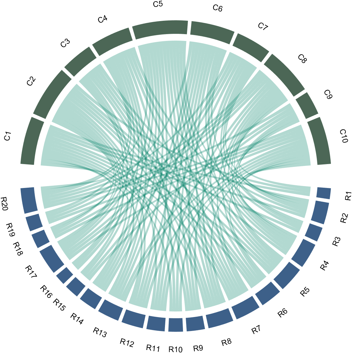
We can modify its Sep attribute:
dataMat=randi([0,1],[20,10]);
% use Sep to decrease space (separation)
% 使用 sep 减小空隙
CC=chordChart(dataMat,'Sep',1/120);
CC=CC.draw();
7 Modify Text Direction
dataMat=randi([0,1],[20,10]);
% use Sep to decrease space (separation)
% 使用 sep 减小空隙
CC=chordChart(dataMat,'Sep',1/120);
CC=CC.draw();
CC.tickState('on')
% version 1.7.0更新
% 函数labelRatato用来旋转标签
% The function labelRatato is used to rotate the label
CC.labelRotate('on')
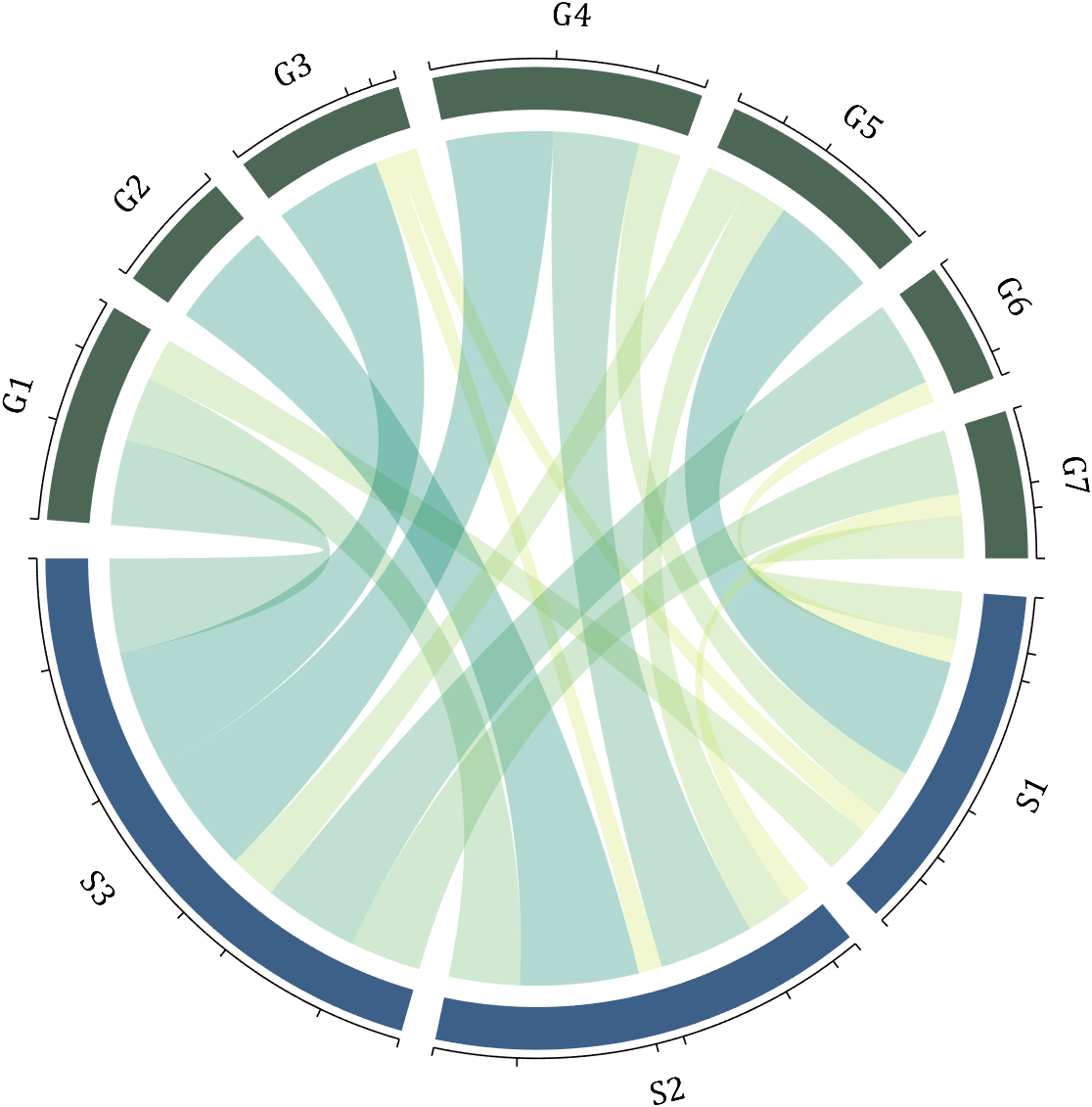
8 Add Tick Labels
dataMat=[2 0 1 2 5 1 2;
3 5 1 4 2 0 1;
4 0 5 5 2 4 3];
colName={'G1','G2','G3','G4','G5','G6','G7'};
rowName={'S1','S2','S3'};
CC=chordChart(dataMat,'rowName',rowName,'colName',colName);
CC=CC.draw();
CC.setFont('FontSize',17,'FontName','Cambria')
% 显示刻度和数值
% Displays scales and numeric values
CC.tickState('on')
CC.tickLabelState('on')
% 调节标签半径
% Adjustable Label radius
CC.setLabelRadius(1.3);
% figure()
% dataMat=[2 0 1 2 5 1 2;
% 3 5 1 4 2 0 1;
% 4 0 5 5 2 4 3];
% dataMat=dataMat+rand(3,7);
% dataMat(dataMat<1)=0;
%
% CC=chordChart(dataMat,'rowName',rowName,'colName',colName);
% CC=CC.draw();
% CC.setFont('FontSize',17,'FontName','Cambria')
%
% % 显示刻度和数值
% % Displays scales and numeric values
% CC.tickState('on')
% CC.tickLabelState('on')
%
% % 调节标签半径
% % Adjustable Label radius
% CC.setLabelRadius(1.4);
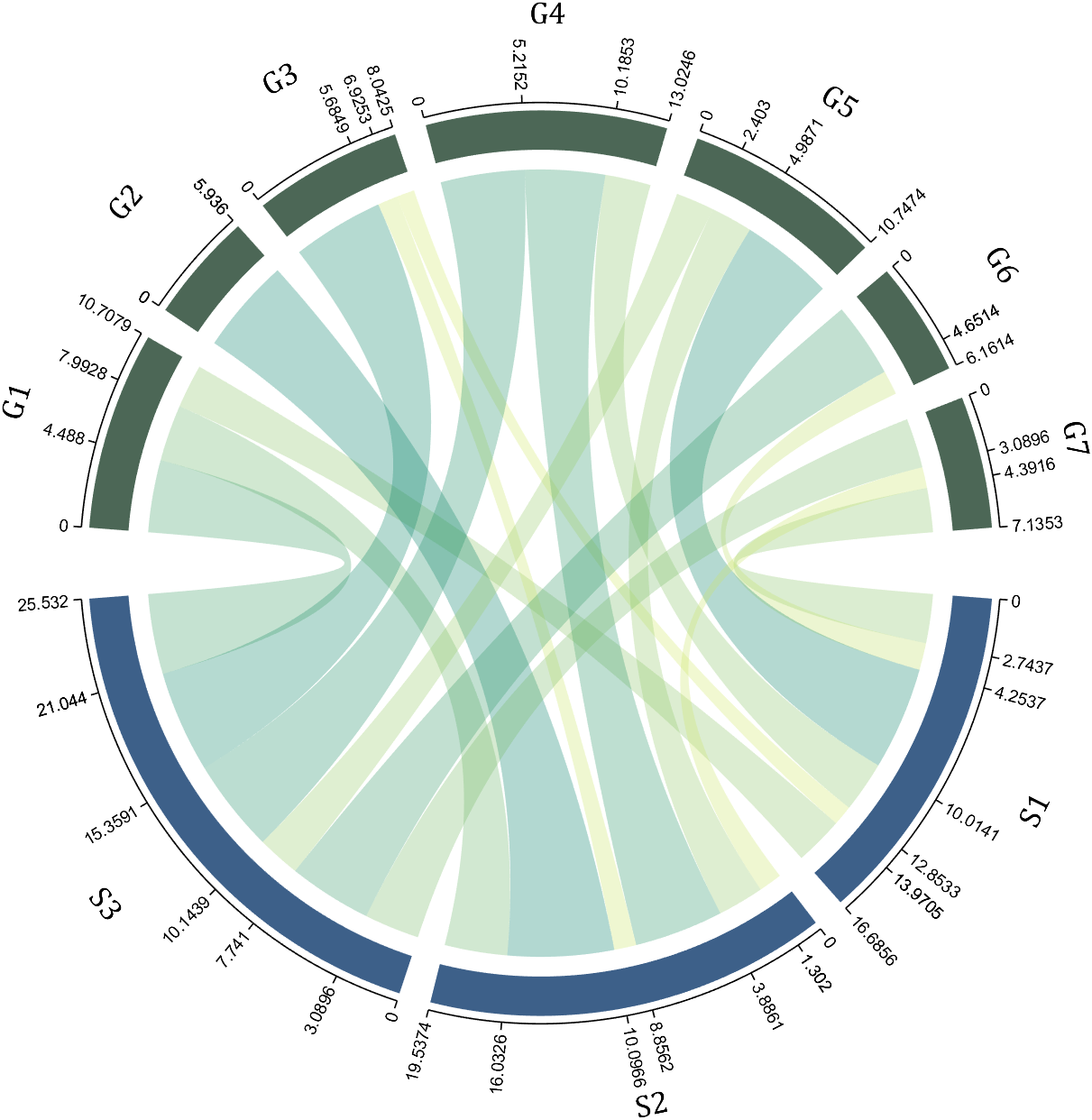
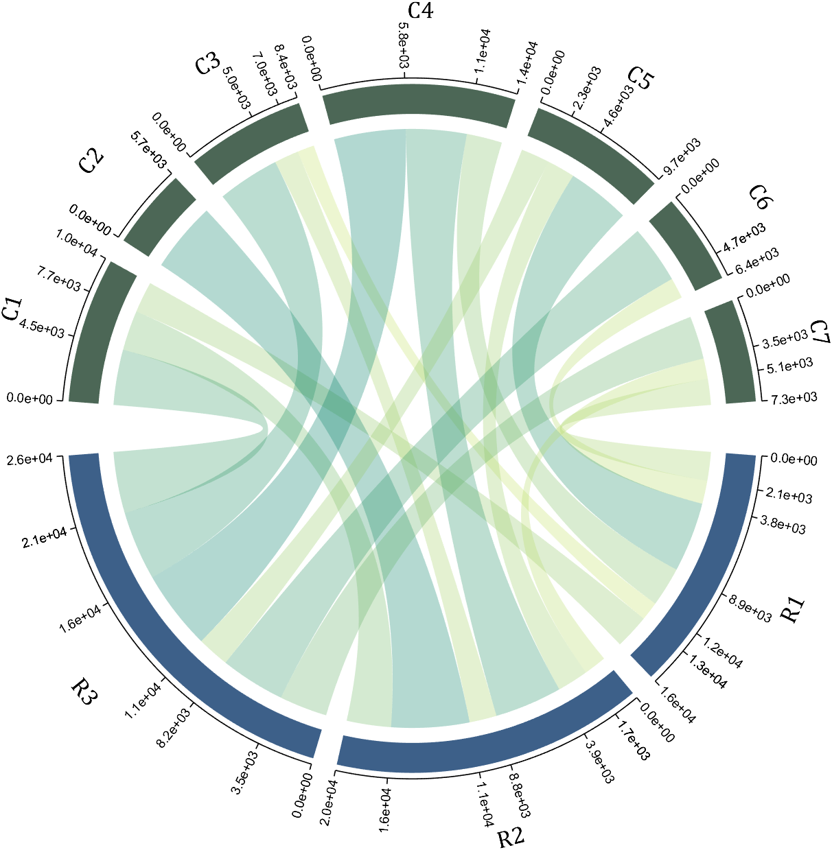
9 Custom Tick Label Format
A function handle is required to input numeric output strings. The format can be set through the setTickLabelFormat function, such as Scientific notation:
dataMat=[2 0 1 2 5 1 2;
3 5 1 4 2 0 1;
4 0 5 5 2 4 3];
dataMat=dataMat+rand(3,7);
dataMat(dataMat<1)=0;
dataMat=dataMat.*1000;
CC=chordChart(dataMat);
CC=CC.draw();
CC.setFont('FontSize',17,'FontName','Cambria')
% 显示刻度和数值
% Displays scales and numeric values
CC.tickState('on')
CC.tickLabelState('on')
% 调节标签半径
% Adjustable Label radius
CC.setLabelRadius(1.4);
% 调整数值字符串格式
% Adjust numeric string format
CC.setTickLabelFormat(@(x)sprintf('%0.1e',x))
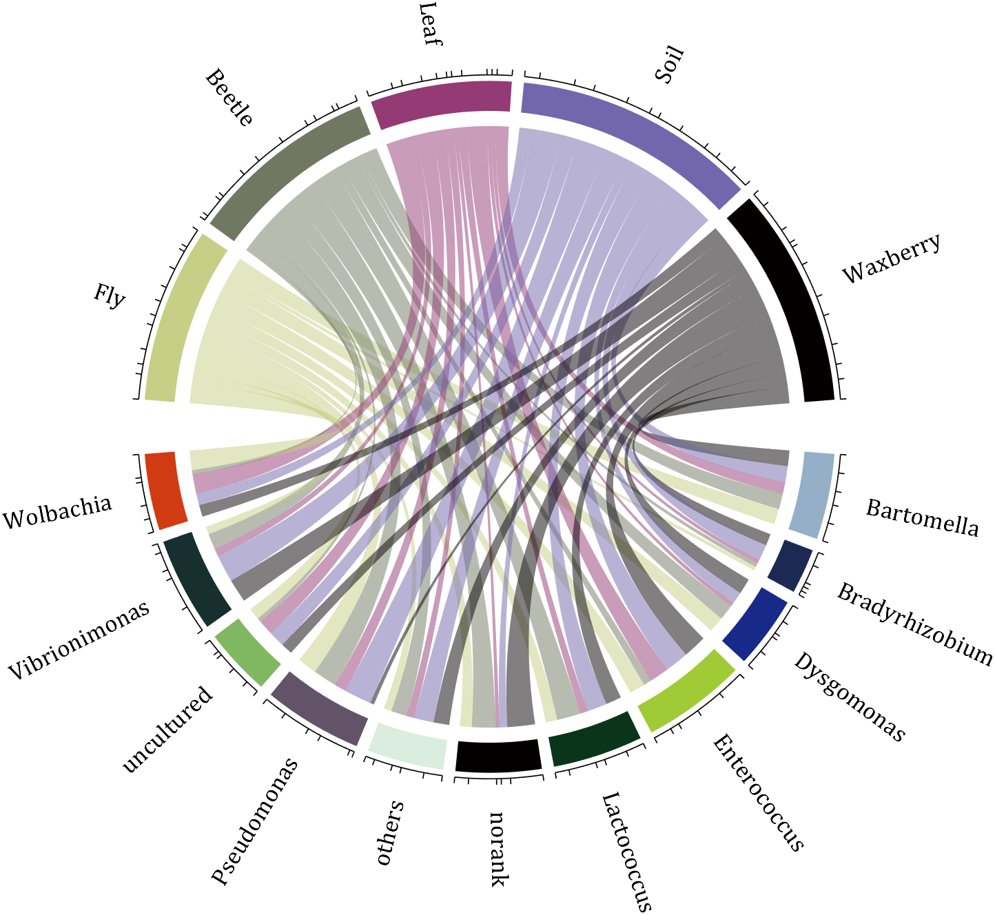
10 A Demo
rng(2)
dataMat=randi([1,7],[11,5]);
colName={'Fly','Beetle','Leaf','Soil','Waxberry'};
rowName={'Bartomella','Bradyrhizobium','Dysgomonas','Enterococcus',...
'Lactococcus','norank','others','Pseudomonas','uncultured',...
'Vibrionimonas','Wolbachia'};
CC=chordChart(dataMat,'rowName',rowName,'colName',colName,'Sep',1/80);
CC=CC.draw();
% 修改上方方块颜色(Modify the color of the blocks above)
CListT=[0.7765 0.8118 0.5216;0.4431 0.4706 0.3843;0.5804 0.2275 0.4549;
0.4471 0.4039 0.6745;0.0157 0 0 ];
for i=1:5
CC.setSquareT_N(i,'FaceColor',CListT(i,:))
end
% 修改下方方块颜色(Modify the color of the blocks below)
CListF=[0.5843 0.6863 0.7843;0.1098 0.1647 0.3255;0.0902 0.1608 0.5373;
0.6314 0.7961 0.2118;0.0392 0.2078 0.1059;0.0157 0 0 ;
0.8549 0.9294 0.8745;0.3882 0.3255 0.4078;0.5020 0.7216 0.3843;
0.0902 0.1843 0.1804;0.8196 0.2314 0.0706];
for i=1:11
CC.setSquareF_N(i,'FaceColor',CListF(i,:))
end
% 修改弦颜色(Modify chord color)
for i=1:5
for j=1:11
CC.setChordMN(j,i,'FaceColor',CListT(i,:),'FaceAlpha',.5)
end
end
CC.tickState('on')
CC.labelRotate('on')
CC.setFont('FontSize',17,'FontName','Cambria')
Hope to have your Reviews and Stars!!!
↓ ↓ ↓ ↓ ↓ ↓ ↓ ↓ ↓ ↓
↑ ↑ ↑ ↑ ↑ ↑ ↑ ↑ ↑ ↑
Most of my projects are the tension between what exists and what I must create to make the project work. The more I leverage what exists, the faster I can complete my project in a shorter amount of time. I often find out later in the process that a MATLAB function already exists and has existed for 10 releases. The faster that I discover built-in functions, the faster I can get to the new stuff that I have to invent.
I asked the AI Chat Playground why to use MATLAB's builtin functions and I got some interesting ideas. What are your thoughts?
AI Chat Playground:
- Efficiency and Performance: MATLAB's built-in functions are highly optimized for performance. They are written in optimized and compiled languages like C or C++, which means they run faster than equivalent functions written directly in MATLAB language. When you use these functions, your code can execute more efficiently, which is especially beneficial for handling large datasets or complex mathematical computations.
- Reliability and Stability: Built-in functions have been rigorously tested and debugged by the developers at MathWorks (the company behind MATLAB). They are less likely to contain errors compared to custom-written code, which means you can rely on them to produce accurate and consistent results.
- Ease of Use: Built-in functions are designed to be user-friendly, with clear documentation and support materials available. This can make it easier to perform complex operations without needing a deep understanding of the underlying algorithms. It also reduces the amount of code you need to write and debug, saving time and reducing the potential for errors.
- Compatibility: Built-in functions are updated alongside MATLAB itself, ensuring compatibility with new features and versions of the software. Using built-in functions can help ensure that your code continues to work correctly as MATLAB evolves.
- Advanced Features: MATLAB’s built-in functions often include advanced features and options that are not readily available or would be difficult to implement on your own. For example, MATLAB’s mathematical functions can handle a wide range of special cases and data types, providing more flexibility than custom implementations.
- Community and Support: Using built-in functions means you're working with standard tools recognized by the MATLAB community. This can make it easier to get help from other users or from MathWorks support, as more people will be familiar with the functionality and potential issues of these functions.
We are thrilled to announce the launch of a brand-new area within the MATLAB Central community – 'Discussions'. This exciting addition is designed to foster a stronger and more connected community.
Discover the 'Tips & Tricks' Channel
At the heart of 'Discussions' is the 'Tips & Tricks' channel. This is your ultimate destination for both sharing and discovering the best MATLAB tips.
Whether you're a seasoned MATLAB user with wisdom to share or a newcomer seeking advice, this channel is your platform. Here, you can post your own insights, ask for guidance on specific topics, and uncover hidden gems that can transform your MATLAB experience. It's more than just a channel; it's a community learning together; it’s your community blog!
More Than Just Tips
The 'Discussions' area offers much more. Explore the 'Ideas'channel to share and debate innovative product ideas. Dive into the 'Fun'channel to enjoy memes and light-hearted content with fellow MATLAB enthusiasts. Or wander into 'Off Topic'for intriguing discussions that might not be related to MATLAB.
Follow the channels!
We highly encourage every member of the MATLAB Central community to follow the channels you are interested in and participate in 'Discussions'. Together, we can achieve more, learn more, and connect more.

Given a vector v whose order we would like to randomly permute, many would perform the permutation by explicitly querying the length/size of v, e.g.,
I=randperm(numel(v));
v=v(I);
However, one can instead do as follows, avoiding the size query.
v=v(randperm(end))
Analogous things can be done with matrices, e.g.,
A=A(randperm(end), randperm(end));
s = ['M','A','T','L','A','B']
9%
char([77,65,84,76,65,66])
7%
"MAT" + "LAB"
21%
upper(char('matlab' - '0' + 48))
17%
fliplr("BALTAM")
17%
rot90(rot90('BALTAM'))
30%
2929 个投票
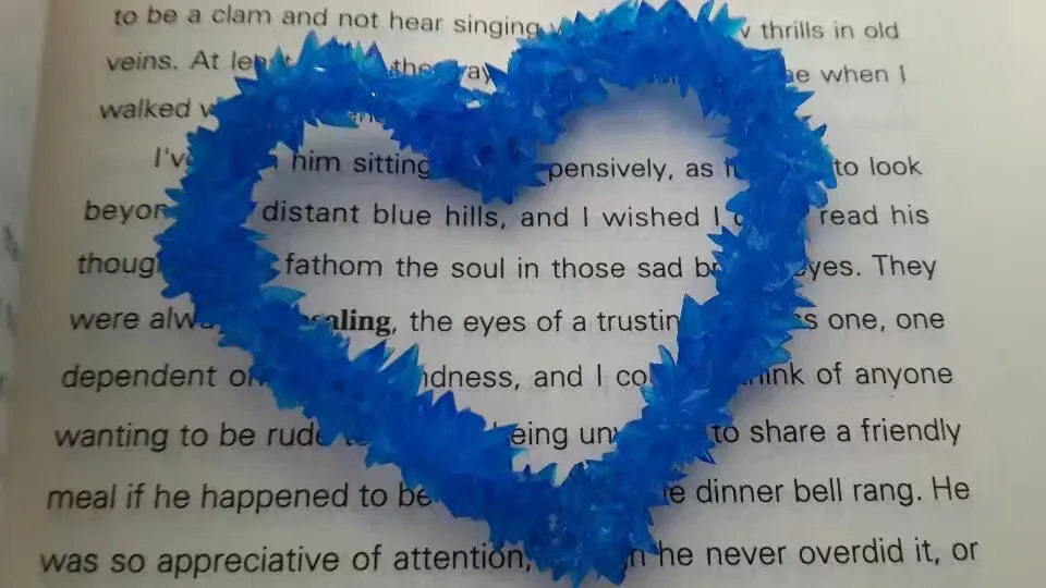
The creativity comes from the copper sulfate crystal heart made in junior high school. Copper sulfate is a triclinic crystal, and the same structure was not used here for convenience in drawing.
Part 1. Coordinate transformation
To draw a crystal heart, one must first be able to draw crystal clusters. To draw a crystal cluster, one must first be able to draw a crystal. To draw a crystal, we need this kind of structure:
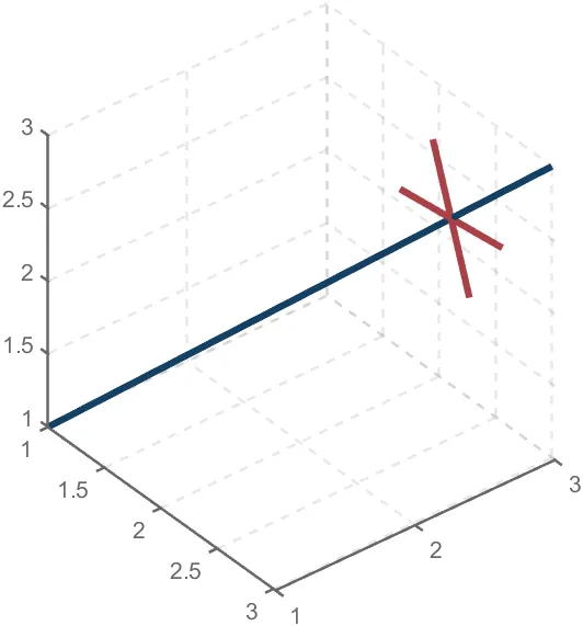
We first need a point with a certain distance from the straight line and a perpendicular point of cutPnt, which is very easy to find, for example, cutPnt=[x0, y0, z0]; The direction of the central axis is V=[x1, y1, z1]; If the distance to the straight line is L, the following points clearly meet the conditions:
v2=[z1,z1,-x1-y1];
v2=v2./norm(v2).*L;
pnt=cutPnt+v2;
But finding only one point is not enough. We need to find four points, and each point is obtained by rotating the previous point around a straight line by  degrees. Therefore, we need to obtain our point rotation transformation matrix around a straight line
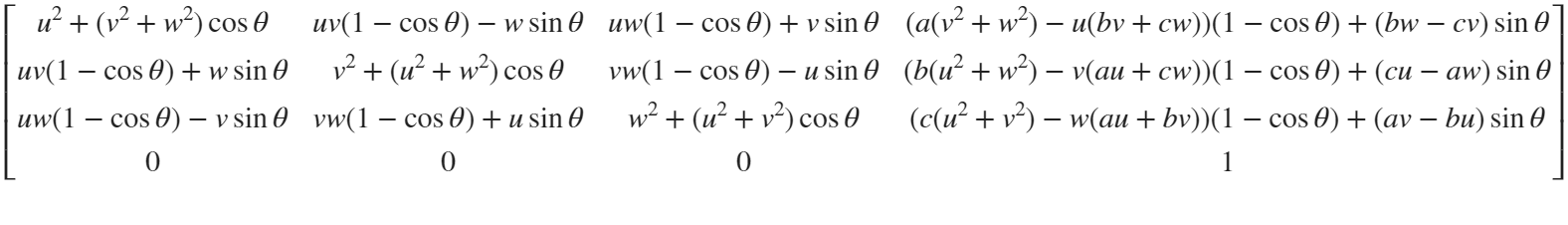
quite complex,right?
rotateMat=[u^2+(v^2+w^2)*cos(theta) , u*v*(1-cos(theta))-w*sin(theta), u*w*(1-cos(theta))+v*sin(theta), (a*(v^2+w^2)-u*(b*v+c*w))*(1-cos(theta))+(b*w-c*v)*sin(theta);
u*v*(1-cos(theta))+w*sin(theta), v^2+(u^2+w^2)*cos(theta) , v*w*(1-cos(theta))-u*sin(theta), (b*(u^2+w^2)-v*(a*u+c*w))*(1-cos(theta))+(c*u-a*w)*sin(theta);
u*w*(1-cos(theta))-v*sin(theta), v*w*(1-cos(theta))+u*sin(theta), w^2+(u^2+v^2)*cos(theta) , (c*(u^2+v^2)-w*(a*u+b*v))*(1-cos(theta))+(a*v-b*u)*sin(theta);
0 , 0 , 0 , 1];
Where [u, v, w] is the directional unit vector, and [a, b, c] is the initial coordinate of the axis:
Part 2. Crystal Cluster Drawing
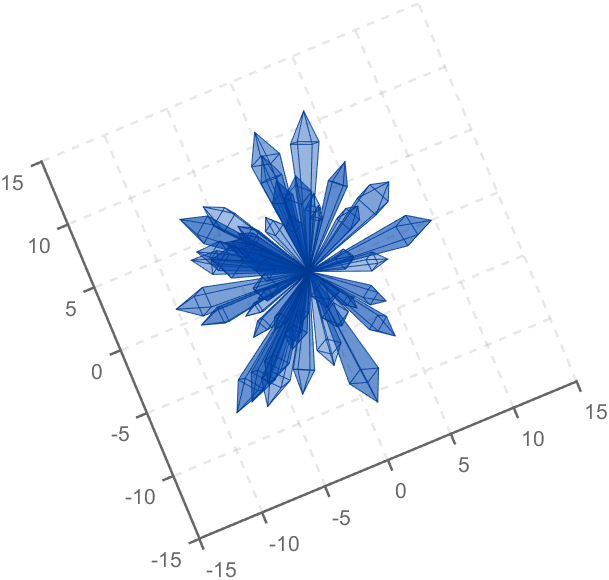
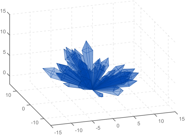
function crystall
hold on
for i=1:50
len=rand(1)*8+5;
tempV=rand(1,3)-0.5;
tempV(3)=abs(tempV(3));
tempV=tempV./norm(tempV).*len;
tempEpnt=tempV;
drawCrystal([0 0 0],tempEpnt,pi/6,0.8,0.1,rand(1).*0.2+0.2)
disp(i)
end
ax=gca;
ax.XLim=[-15,15];
ax.YLim=[-15,15];
ax.ZLim=[-2,15];
grid on
ax.GridLineStyle='--';
ax.LineWidth=1.2;
ax.XColor=[1,1,1].*0.4;
ax.YColor=[1,1,1].*0.4;
ax.ZColor=[1,1,1].*0.4;
ax.DataAspectRatio=[1,1,1];
ax.DataAspectRatioMode='manual';
ax.CameraPosition=[-67.6287 -204.5276 82.7879];
function drawCrystal(Spnt,Epnt,theta,cl,w,alpha)
%plot3([Spnt(1),Epnt(1)],[Spnt(2),Epnt(2)],[Spnt(3),Epnt(3)])
mainV=Epnt-Spnt;
cutPnt=cl.*(mainV)+Spnt;
cutV=[mainV(3),mainV(3),-mainV(1)-mainV(2)];
cutV=cutV./norm(cutV).*w.*norm(mainV);
cornerPnt=cutPnt+cutV;
cornerPnt=rotateAxis(Spnt,Epnt,cornerPnt,theta);
cornerPntSet(1,:)=cornerPnt';
for ii=1:3
cornerPnt=rotateAxis(Spnt,Epnt,cornerPnt,pi/2);
cornerPntSet(ii+1,:)=cornerPnt';
end
F = [1,3,4;1,4,5;1,5,6;1,6,3;...
2,3,4;2,4,5;2,5,6;2,6,3];
V = [Spnt;Epnt;cornerPntSet];
patch('Faces',F,'Vertices',V,'FaceColor',[0 71 177]./255,...
'FaceAlpha',alpha,'EdgeColor',[0 71 177]./255.*0.8,...
'EdgeAlpha',0.6,'LineWidth',0.5,'EdgeLighting',...
'gouraud','SpecularStrength',0.3)
end
function newPnt=rotateAxis(Spnt,Epnt,cornerPnt,theta)
V=Epnt-Spnt;V=V./norm(V);
u=V(1);v=V(2);w=V(3);
a=Spnt(1);b=Spnt(2);c=Spnt(3);
cornerPnt=[cornerPnt(:);1];
rotateMat=[u^2+(v^2+w^2)*cos(theta) , u*v*(1-cos(theta))-w*sin(theta), u*w*(1-cos(theta))+v*sin(theta), (a*(v^2+w^2)-u*(b*v+c*w))*(1-cos(theta))+(b*w-c*v)*sin(theta);
u*v*(1-cos(theta))+w*sin(theta), v^2+(u^2+w^2)*cos(theta) , v*w*(1-cos(theta))-u*sin(theta), (b*(u^2+w^2)-v*(a*u+c*w))*(1-cos(theta))+(c*u-a*w)*sin(theta);
u*w*(1-cos(theta))-v*sin(theta), v*w*(1-cos(theta))+u*sin(theta), w^2+(u^2+v^2)*cos(theta) , (c*(u^2+v^2)-w*(a*u+b*v))*(1-cos(theta))+(a*v-b*u)*sin(theta);
0 , 0 , 0 , 1];
newPnt=rotateMat*cornerPnt;
newPnt(4)=[];
end
end
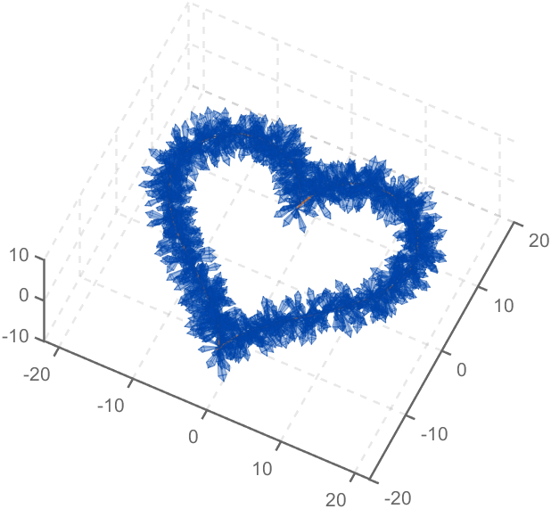
Part 3. Drawing of Crystal Heart
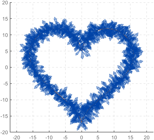
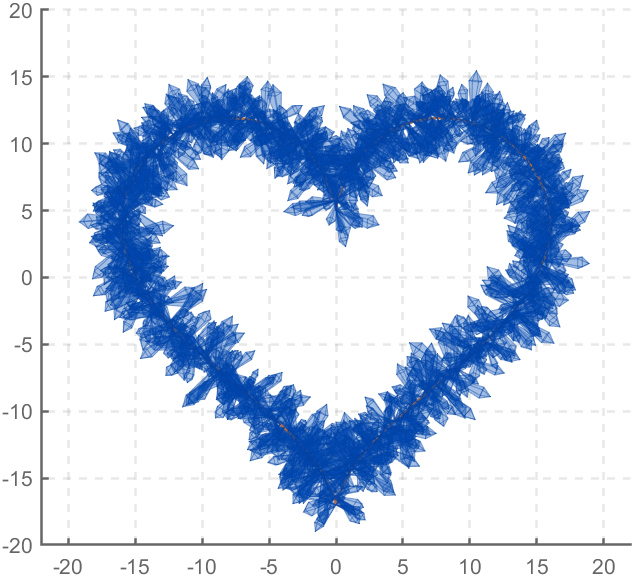
function crystalHeart
clc;clear;close all
hold on
% drawCrystal([1,1,1],[3,3,3],pi/6,0.8,0.14)
sep=pi/8;
t=[0:0.2:sep,sep:0.02:pi-sep,pi-sep:0.2:pi+sep,pi+sep:0.02:2*pi-sep,2*pi-sep:0.2:2*pi];
x=16*sin(t).^3;
y=13*cos(t)-5*cos(2*t)-2*cos(3*t)-cos(4*t);
z=zeros(size(t));
plot3(x,y,z,'Color',[186,110,64]./255,'LineWidth',1)
for i=1:length(t)
for j=1:6
len=rand(1)*2.5+1.5;
tempV=rand(1,3)-0.5;
tempV=tempV./norm(tempV).*len;
tempSpnt=[x(i),y(i),z(i)];
tempEpnt=tempV+tempSpnt;
drawCrystal(tempSpnt,tempEpnt,pi/6,0.8,0.14)
disp([i,j])
end
end
ax=gca;
ax.XLim=[-22,22];
ax.YLim=[-20,20];
ax.ZLim=[-10,10];
grid on
ax.GridLineStyle='--';
ax.LineWidth=1.2;
ax.XColor=[1,1,1].*0.4;
ax.YColor=[1,1,1].*0.4;
ax.ZColor=[1,1,1].*0.4;
ax.DataAspectRatio=[1,1,1];
ax.DataAspectRatioMode='manual';
function drawCrystal(Spnt,Epnt,theta,cl,w)
%plot3([Spnt(1),Epnt(1)],[Spnt(2),Epnt(2)],[Spnt(3),Epnt(3)])
mainV=Epnt-Spnt;
cutPnt=cl.*(mainV)+Spnt;
cutV=[mainV(3),mainV(3),-mainV(1)-mainV(2)];
cutV=cutV./norm(cutV).*w.*norm(mainV);
cornerPnt=cutPnt+cutV;
cornerPnt=rotateAxis(Spnt,Epnt,cornerPnt,theta);
cornerPntSet(1,:)=cornerPnt';
for ii=1:3
cornerPnt=rotateAxis(Spnt,Epnt,cornerPnt,pi/2);
cornerPntSet(ii+1,:)=cornerPnt';
end
F = [1,3,4;1,4,5;1,5,6;1,6,3;...
2,3,4;2,4,5;2,5,6;2,6,3];
V = [Spnt;Epnt;cornerPntSet];
patch('Faces',F,'Vertices',V,'FaceColor',[0 71 177]./255,...
'FaceAlpha',0.2,'EdgeColor',[0 71 177]./255.*0.9,...
'EdgeAlpha',0.25,'LineWidth',0.01,'EdgeLighting',...
'gouraud','SpecularStrength',0.3)
end
function newPnt=rotateAxis(Spnt,Epnt,cornerPnt,theta)
V=Epnt-Spnt;V=V./norm(V);
u=V(1);v=V(2);w=V(3);
a=Spnt(1);b=Spnt(2);c=Spnt(3);
cornerPnt=[cornerPnt(:);1];
rotateMat=[u^2+(v^2+w^2)*cos(theta) , u*v*(1-cos(theta))-w*sin(theta), u*w*(1-cos(theta))+v*sin(theta), (a*(v^2+w^2)-u*(b*v+c*w))*(1-cos(theta))+(b*w-c*v)*sin(theta);
u*v*(1-cos(theta))+w*sin(theta), v^2+(u^2+w^2)*cos(theta) , v*w*(1-cos(theta))-u*sin(theta), (b*(u^2+w^2)-v*(a*u+c*w))*(1-cos(theta))+(c*u-a*w)*sin(theta);
u*w*(1-cos(theta))-v*sin(theta), v*w*(1-cos(theta))+u*sin(theta), w^2+(u^2+v^2)*cos(theta) , (c*(u^2+v^2)-w*(a*u+b*v))*(1-cos(theta))+(a*v-b*u)*sin(theta);
0 , 0 , 0 , 1];
newPnt=rotateMat*cornerPnt;
newPnt(4)=[];
end
end
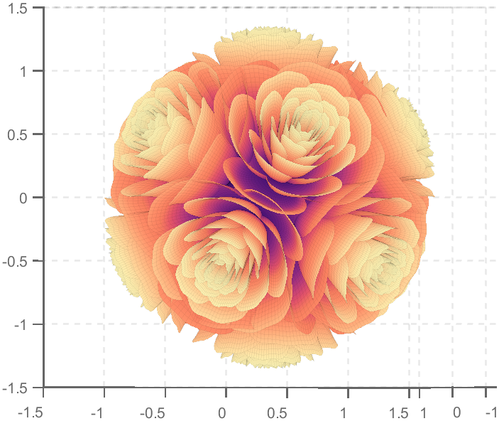
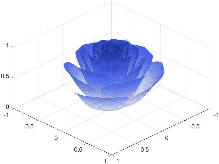
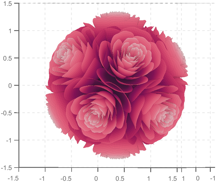
So, how to draw a roseball just like this ?
To begin with, we need to know how to draw a single rose in MATLAB:
function drawrose
set(gca,'CameraPosition',[2 2 2])
hold on
grid on
[x,t]=meshgrid((0:24)./24,(0:0.5:575)./575.*20.*pi+4*pi);
p=(pi/2)*exp(-t./(8*pi));
change=sin(15*t)/150;
u=1-(1-mod(3.6*t,2*pi)./pi).^4./2+change;
y=2*(x.^2-x).^2.*sin(p);
r=u.*(x.*sin(p)+y.*cos(p));
h=u.*(x.*cos(p)-y.*sin(p));
surface(r.*cos(t),r.*sin(t),h,'EdgeAlpha',0.1,...
'EdgeColor',[0 0 0],'FaceColor','interp')
end
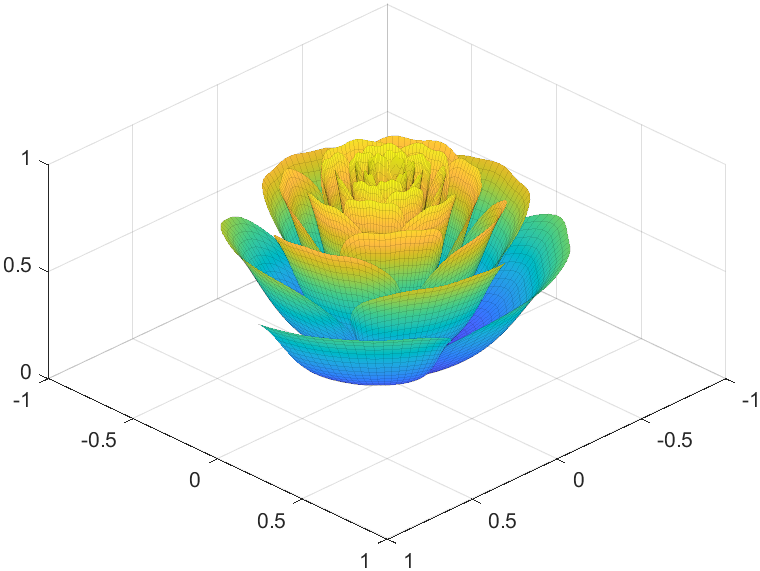
Tts pretty easy, Now we are trying to dye it the desired color:
function drawrose
set(gca,'CameraPosition',[2 2 2])
hold on
grid on
[x,t]=meshgrid((0:24)./24,(0:0.5:575)./575.*20.*pi+4*pi);
p=(pi/2)*exp(-t./(8*pi));
change=sin(15*t)/150;
u=1-(1-mod(3.6*t,2*pi)./pi).^4./2+change;
y=2*(x.^2-x).^2.*sin(p);
r=u.*(x.*sin(p)+y.*cos(p));
h=u.*(x.*cos(p)-y.*sin(p));
map=[0.9176 0.9412 1.0000
0.8353 0.8706 0.9922
0.8196 0.8627 0.9804
0.7020 0.7569 0.9412
0.5176 0.5882 0.9255
0.3686 0.4824 0.9412
0.3059 0.4000 0.9333
0.2275 0.3176 0.8353
0.1216 0.2275 0.6471];
Xi=1:size(map,1);Xq=linspace(1,size(map,1),100);
map=[interp1(Xi,map(:,1),Xq,'linear')',...
interp1(Xi,map(:,2),Xq,'linear')',...
interp1(Xi,map(:,3),Xq,'linear')'];
surface(r.*cos(t),r.*sin(t),h,'EdgeAlpha',0.1,...
'EdgeColor',[0 0 0],'FaceColor','interp')
colormap(map)
end
I try to take colors from real roses and interpolate them to make them more realistic
Then, how can I put these colorful flowers on to a ball ?
We need to place the drawn flowers on each face of the polyhedron sphere through coordinate transformation. Here, we use a regular dodecahedron:
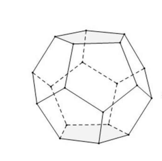
Move the flower using the following rotation formula:
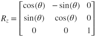
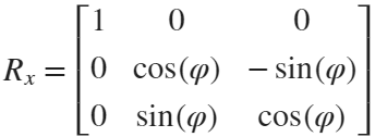
We place a flower on each plane, which means that the angle between every two flowers is 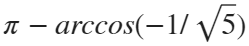 degrees. We can place each flower at the appropriate angle through multiple x-axis rotations and multiple z-axis rotations. The code is as follows:
function roseBall(colorList)
%曲面数据计算
%==========================================================================
[x,t]=meshgrid((0:24)./24,(0:0.5:575)./575.*20.*pi+4*pi);
p=(pi/2)*exp(-t./(8*pi));
change=sin(15*t)/150;
u=1-(1-mod(3.6*t,2*pi)./pi).^4./2+change;
y=2*(x.^2-x).^2.*sin(p);
r=u.*(x.*sin(p)+y.*cos(p));
h=u.*(x.*cos(p)-y.*sin(p));
%颜色映射表
%==========================================================================
hMap=(h-min(min(h)))./(max(max(h))-min(min(h)));
col=size(hMap,2);
if nargin<1
colorList=[0.0200 0.0400 0.3900
0 0.0900 0.5800
0 0.1300 0.6400
0.0200 0.0600 0.6900
0 0.0800 0.7900
0.0100 0.1800 0.8500
0 0.1300 0.9600
0.0100 0.2600 0.9900
0 0.3500 0.9900
0.0700 0.6200 1.0000
0.1700 0.6900 1.0000];
end
colorFunc=colorFuncFactory(colorList);
dataMap=colorFunc(hMap');
colorMap(:,:,1)=dataMap(:,1:col);
colorMap(:,:,2)=dataMap(:,col+1:2*col);
colorMap(:,:,3)=dataMap(:,2*col+1:3*col);
function colorFunc=colorFuncFactory(colorList)
xx=(0:size(colorList,1)-1)./(size(colorList,1)-1);
y1=colorList(:,1);y2=colorList(:,2);y3=colorList(:,3);
colorFunc=@(X)[interp1(xx,y1,X,'linear')',interp1(xx,y2,X,'linear')',interp1(xx,y3,X,'linear')'];
end
%曲面旋转及绘制
%==========================================================================
surface(r.*cos(t),r.*sin(t),h+0.35,'EdgeAlpha',0.05,...
'EdgeColor',[0 0 0],'FaceColor','interp','CData',colorMap)
hold on
surface(r.*cos(t),r.*sin(t),-h-0.35,'EdgeAlpha',0.05,...
'EdgeColor',[0 0 0],'FaceColor','interp','CData',colorMap)
Xset=r.*cos(t);
Yset=r.*sin(t);
Zset=h+0.35;
yaw_z=72*pi/180;
roll_x=pi-acos(-1/sqrt(5));
R_z_2=[cos(yaw_z),-sin(yaw_z),0;
sin(yaw_z),cos(yaw_z),0;
0,0,1];
R_z_1=[cos(yaw_z/2),-sin(yaw_z/2),0;
sin(yaw_z/2),cos(yaw_z/2),0;
0,0,1];
R_x_2=[1,0,0;
0,cos(roll_x),-sin(roll_x);
0,sin(roll_x),cos(roll_x)];
[nX,nY,nZ]=rotateXYZ(Xset,Yset,Zset,R_x_2);
surface(nX,nY,nZ,'EdgeAlpha',0.05,...
'EdgeColor',[0 0 0],'FaceColor','interp','CData',colorMap)
for k=1:4
[nX,nY,nZ]=rotateXYZ(nX,nY,nZ,R_z_2);
surface(nX,nY,nZ,'EdgeAlpha',0.05,...
'EdgeColor',[0 0 0],'FaceColor','interp','CData',colorMap)
end
[nX,nY,nZ]=rotateXYZ(nX,nY,nZ,R_z_1);
for k=1:5
[nX,nY,nZ]=rotateXYZ(nX,nY,nZ,R_z_2);
surface(nX,nY,-nZ,'EdgeAlpha',0.05,...
'EdgeColor',[0 0 0],'FaceColor','interp','CData',colorMap)
end
%--------------------------------------------------------------------------
function [nX,nY,nZ]=rotateXYZ(X,Y,Z,R)
nX=zeros(size(X));
nY=zeros(size(Y));
nZ=zeros(size(Z));
for i=1:size(X,1)
for j=1:size(X,2)
v=[X(i,j);Y(i,j);Z(i,j)];
nv=R*v;
nX(i,j)=nv(1);
nY(i,j)=nv(2);
nZ(i,j)=nv(3);
end
end
end
%axes属性调整
%==========================================================================
ax=gca;
grid on
ax.GridLineStyle='--';
ax.LineWidth=1.2;
ax.XColor=[1,1,1].*0.4;
ax.YColor=[1,1,1].*0.4;
ax.ZColor=[1,1,1].*0.4;
ax.DataAspectRatio=[1,1,1];
ax.DataAspectRatioMode='manual';
ax.CameraPosition=[-6.5914 -24.1625 -0.0384];
end

TRY DIFFERENT COLORS !!
colorList1=[0.2000 0.0800 0.4300
0.2000 0.1300 0.4600
0.2000 0.2100 0.5000
0.2000 0.2800 0.5300
0.2000 0.3700 0.5800
0.1900 0.4500 0.6200
0.2000 0.4800 0.6400
0.1900 0.5400 0.6700
0.1900 0.5700 0.6900
0.1900 0.7500 0.7800
0.1900 0.8000 0.8100
];
colorList2=[0.1300 0.1000 0.1600
0.2000 0.0900 0.2000
0.2800 0.0800 0.2300
0.4200 0.0800 0.3000
0.5100 0.0700 0.3400
0.6600 0.1200 0.3500
0.7900 0.2200 0.4000
0.8800 0.3500 0.4700
0.9000 0.4500 0.5400
0.8900 0.7800 0.7900
];
colorList3=[0.3200 0.3100 0.7600
0.3800 0.3400 0.7600
0.5300 0.4200 0.7500
0.6400 0.4900 0.7300
0.7200 0.5500 0.7200
0.7900 0.6100 0.7100
0.9100 0.7100 0.6800
0.9800 0.7600 0.6700
];
colorList4=[0.2100 0.0900 0.3800
0.2900 0.0700 0.4700
0.4000 0.1100 0.4900
0.5500 0.1600 0.5100
0.7500 0.2400 0.4700
0.8900 0.3200 0.4100
0.9700 0.4900 0.3700
1.0000 0.5600 0.4100
1.0000 0.6900 0.4900
1.0000 0.8200 0.5900
0.9900 0.9200 0.6700
0.9800 0.9500 0.7100];
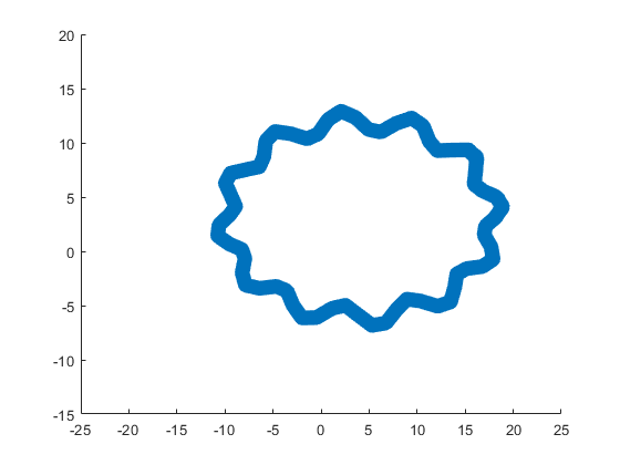
Let us consider how to draw a Happy Sheep. A Happy Sheep was introduced in the MATLAB Mini Hack contest: Happy Sheep!
In this contest there was the strict limitation on the code length. So the code of the Happy Sheep is very compact and is only 280 characters long. We will analyze the process of drawing the Happy Sheep in MATLAB step by step. The explanations of the even more compact version of the code of the same sheep are given below.
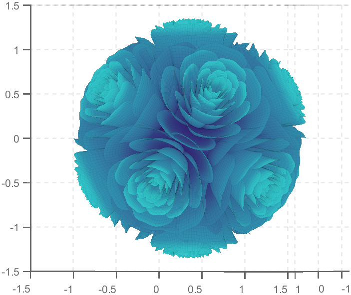
So, how to draw a sheep? It is very easy. We could notice that usually a sheep is covered by crimped wool. Therefore, a sheep could be painted using several geometrical curves of similar types. Of course, then it will be an abstract model of the real sheep. Let us select two mathematical curves, which are the most appropriate for our goal. They are an ellipse for smooth parts of the sheep and an ellipse combined with a rose for woolen parts of the sheep.
Let us recall the mathematical formulas of these curves. A parametric representation of the standard ellipse is the following:
Also we will use the following parametric representation of the rose (rhodonea) curve:
This curve was named by the mathematician Guido Grandi.
Let us combine them in one curve and add possible shifts:
Now if we would like to create an ellipse, we will set  and
and  . If we would like to create a rose, we will set
  and
and  . If we would like to shift our curve, we will set
  and
and  to the required values. Of course, we could set all non-zero parameters to combine both chosen curves and use the shifts.
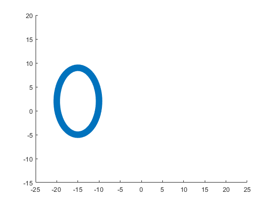
Let us describe how to create these curves using the MATLAB code. To make the code more compact, it is possible to program both formulas for the combined curve in one line using the anonymous function. We could make the code more compact using the function handles for sine and cosine functions. Then the MATLAB code for an example of the ellipse curve will be the following.
% Handles
s=@sin;
c=@cos;
% Ellipse + Polar Rose
F=@(t,a,f) a(1)*f(t)+s(a(2)*t).*f(t)+a(3);
% Angles
t=0:.1:7;
% Parameters
E = [5 7;0 0;0 0];
% Painting
figure;
plot(F(t,E(:,1),c),F(t,E(:,2),s),'LineWidth',10);
axis equal
The parameter t varies from 0 to 7, which is the nearest integer greater than  , with the step 0.1. The result of this code is the following ellipse curve with
  and
and  .
.
This ellipse is described by the following parametric equations:
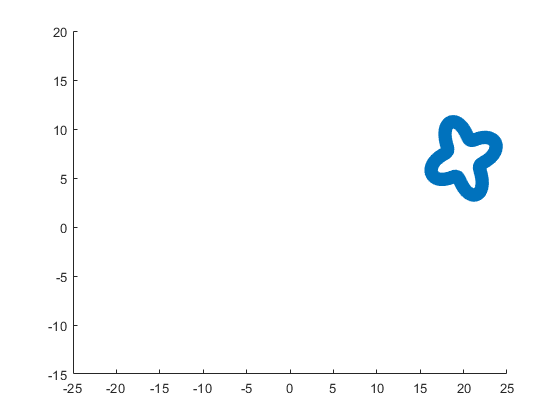
The MATLAB code for an example of the rose curve will be the following.
% Handles
s=@sin;
c=@cos;
% Ellipse + Polar Rose
F=@(t,a,f) a(1)*f(t)+s(a(2)*t).*f(t)+a(3);
% Angles
t=0:.1:7;
% Parameters
R = [0 0;4 4;0 0];
% Painting
figure;
plot(F(t,R(:,1),c),F(t,R(:,2),s),'LineWidth',10);
axis equal
The result of this code is the following rose curve with  and
and  .
.
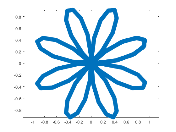
This rose is described by the following parametric equations:
Obviously, now we are ready to draw main parts of our sheep! As we reproduce an abstract model of the sheep, let us select the following main parts for the representation: head, eyes, hoofs, body, crown, and tail. We will use ellipses for the first three parts in this list and ellipses combined with roses for the last three ones.
First let us describe drawing of each part independently.
The following MATLAB code will be used to do this.
% Handles
s=@sin;
c=@cos;
% Ellipse + Polar Rose
F=@(t,a,f) a(1)*f(t)+s(a(2)*t).*f(t)+a(3);
% Angles
t=0:.1:7;
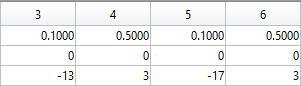
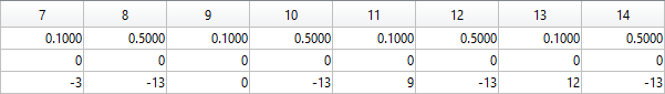
% Parameters
Head = 1;
Eyes = 2:3;
Hoofs = 4:7;
Body = 8;
Crown = 9;
Tail = 10;
G=-13;
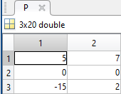
P=[5 7 repmat([.1 .5],1,6) 6 4 14 9 3 3;zeros(1,14) 8 8 12 12 4 4;...
-15 2 G 3 -17 3 -3 G 0 G 9 G 12 G -15 12 4 3 20 7];
% Painting
figure;
hold;
for i=Head
plot(F(t,P(:,2*i-1),c),F(t,P(:,2*i),s),'LineWidth',10);
end
axis([-25 25 -15 20]);
figure;
hold;
for i=Eyes
plot(F(t,P(:,2*i-1),c),F(t,P(:,2*i),s),'LineWidth',10);
end
axis([-25 25 -15 20]);
figure;
hold;
for i=Hoofs
plot(F(t,P(:,2*i-1),c),F(t,P(:,2*i),s),'LineWidth',10);
end
axis([-25 25 -15 20]);
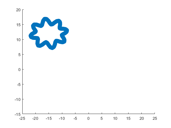
figure;
hold;
for i=Body
plot(F(t,P(:,2*i-1),c),F(t,P(:,2*i),s),'LineWidth',10);
end
axis([-25 25 -15 20]);
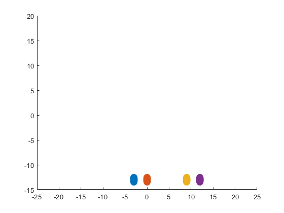
figure;
hold;
for i=Crown
plot(F(t,P(:,2*i-1),c),F(t,P(:,2*i),s),'LineWidth',10);
end
axis([-25 25 -15 20]);
figure;
hold;
for i=Tail
plot(F(t,P(:,2*i-1),c),F(t,P(:,2*i),s),'LineWidth',10);
end
axis([-25 25 -15 20]);
The parameters  ,
,  ,
,  ,
,  ,
,  , and
, and  are written in the different submatrices of the matrix P. The code generates the following curves to illustrate the different parts of our sheep.
The following ellipse describes the head of the sheep.
The following submatrix of the matrix P represents its parameters.
The parametric equations of the head are the following:
The following ellipses describe the eyes of the sheep.
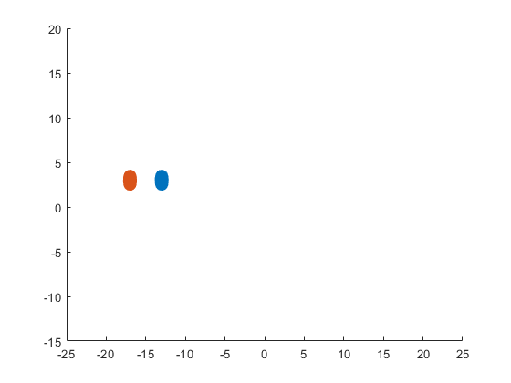
The following submatrices of the matrix P represent their parameters.
The parametric equations of the left and right eyes correspondingly are the following:
The following ellipses describe the hoofs of the sheep.
The following submatrices of the matrix P represent their parameters.
The parametric equations of the right front, left front, right hind, and left hind hoofs correspondingly are the following:
The following ellipse combined with the rose describes the crown of the sheep.
The following submatrix of the matrix P represents its parameters.
The parametric equations of the crown are the following:
The following ellipse combined with the rose describes the body of the sheep.
The following submatrix of the matrix P represents its parameters.
The parametric equations of the body are the following:
The following ellipse combined with the rose describes the tail of the sheep.
The following submatrix of the matrix P represents its parameters.
The parametric equations of the tail are the following:
Now all the parts of our sheep should be put together! It is very easy because all the parts are described by the same equations with different parameters.
The following code helps us to accomplish this goal and ultimately draw a Happy Sheep in MATLAB!
% Happy Sheep!
% By Victoria A. Sablina
% Handles
s=@sin;
c=@cos;
% Ellipse + Rose
F=@(t,a,f) a(1)*f(t)+s(a(2)*t).*f(t)+a(3);
% Angles
t=0:.1:7;
% Parameters
% Head (1:2)
% Eyes (3:6)
% Hoofs (7:14)
% Crown (15:16)
% Body (17:18)
% Tail (19:20)
G=-13;
P=[5 7 repmat([.1 .5],1,6) 6 4 14 9 3 3;zeros(1,14) 8 8 12 12 4 4;...
-15 2 G 3 -17 3 -3 G 0 G 9 G 12 G -15 12 4 3 20 7];
% Painting
hold;
for i=1:10
plot(F(t,P(:,2*i-1),c),F(t,P(:,2*i),s),'LineWidth',10);
end
This code is even more compact than the original code from the contest. It is only 253 instead of 280 characters long and generates the same Happy Sheep!
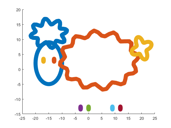
Our sheep is happy, because of becoming famous in the MATLAB community, a star!
Congratulations! Now you know how to draw a Happy Sheep in MATLAB!
Thank you for reading!
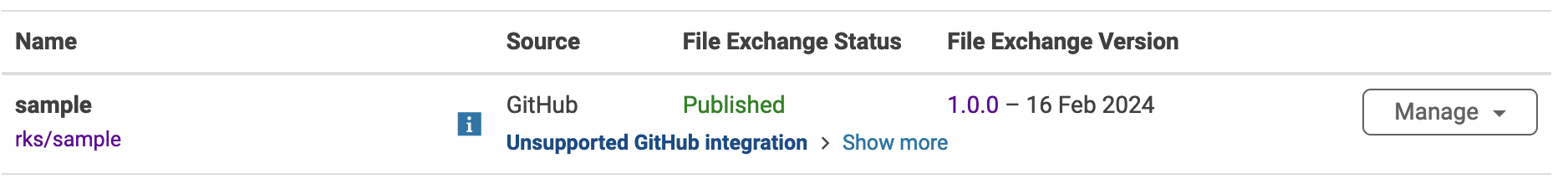
The File Exchange team is thrilled to introduce a more streamlined approach to working with GitHub and File Exchange - the MATLAB and Simulink Integration for GitHub!
Key Enhancements:
- Improves the existing connection between File Exchange and GitHub, ensuring quicker reflection of changes made in GitHub within File Exchange.
- Aligns with GitHub's standard and supported approach to building integrations.
Action Required for File Exchange Contributors!
If you are a File Exchange contributor and have linked any submissions to GitHub, it is essential to install the App.
Starting April 16, 2024, your File Exchange submissions will no longer update automatically unless you take the following steps:
2. Follow the prompts on the page to install MATLAB and Simulink Integration for GitHub.
3. Complete the necessary steps in GitHub.
4. Return to the My File Exchange page and verify the installation.
If you prefer your File Exchange submission not to update automatically from GitHub, no action is required. Users will still be able to find and download your submissions. However, to release a new version of your code, you must either install the GitHub App or disconnect from GitHub and manually upload new versions of your code.
Should you have any questions or encounter issues with the App, please feel free to comment on this post!
I asked my question in the general forum and a few minutes later it was deleted. Perhaps this is a better place?
Rather than using my German regional forum (as I do not speak German), I want to ask questions in an international English-speaking forum. Presumably there should be an international English forum for everyone around the world, as English is the first or second language of everyone who has gone to school. Where is it?
Big congratulations to @VBBV for achieving the remarkable milestone of 3,000 reputation points, earning the prestigious title of Editor within our community.
This achievement is a testament to @VBBV's exceptional contributions and steadfast commitment to the community. These efforts have also been endorsed by fellow top contributors, underscoring the value and impact of @VBBV's expertise.
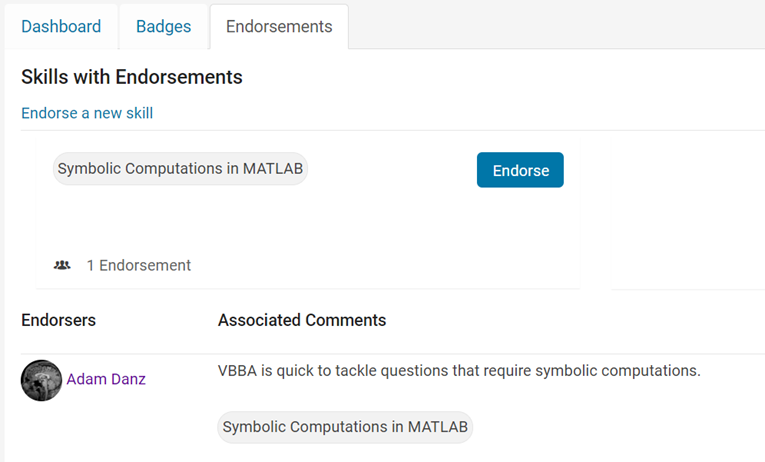
Welcome to the Editors' Club, @VBBV – we are excited to witness and support your continued journey and influence within our community!
eye(3) - diag(ones(1,3))
11%
0 ./ ones(3)
9%
cos(repmat(pi/2, [3,3]))
16%
zeros(3)
20%
A(3, 3) = 0
32%
mtimes([1;1;0], [0,0,0])
12%
3009 个投票
MATLAB O/X Quiz
Answer BEFORE Googling!
- An infinite loop can be made using "for".
- "A == A" is always true.
- "round(2.5)" is 3.
- "round(-0.5)" is 0.
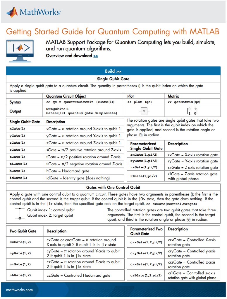
MATLAB Support Package for Quantum Computing lets you build, simulate, and run quantum algorithms.
Check out the Cheat Sheet here!
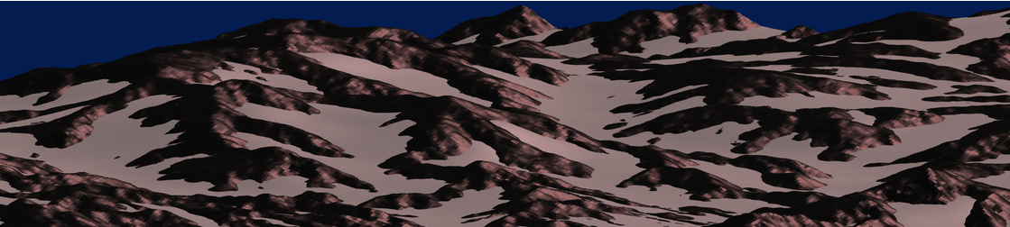
I think that MATLAB's Flipbook Mini Hack had quite some inspiring entries. My work largely deals with digital elevation models (DEMs). Hence I really liked the random renderings of landscapes, in particular this one written by Tim which inspired me to adopt the code and apply to the example data that comes with my software TopoToolbox. The results and code are shown here.
您也可以从以下列表中选择网站:
美洲
- América Latina (Español)
- Canada (English)
- United States (English)
欧洲
- Belgium (English)
- Denmark (English)
- Deutschland (Deutsch)
- España (Español)
- Finland (English)
- France (Français)
- Ireland (English)
- Italia (Italiano)
- Luxembourg (English)
- Netherlands (English)
- Norway (English)
- Österreich (Deutsch)
- Portugal (English)
- Sweden (English)
- Switzerland
- United Kingdom(English)
亚太
- Australia (English)
- India (English)
- New Zealand (English)
- 中国
- 日本Japanese (日本語)
- 한국Korean (한국어)