搜索
As of R2026a, only the Apple Silicon series is supported.
My Intel Mac dates to June 2020; the M1 series was released in November 2020.
So we got only 5 years of use before MATLAB gave up on us. 2 years (R2023b) since the native M1 version was introduced.
I don't exactly have a spare $2500 to spend on a new iMac -- especially not for one that has a maximum of 32 gigabytes of memory when my current system has 128 gigabytes of memory.
I remain disappointed that Mathworks did not continue Intel support for longer.
We are nearly at the anniversary of The Great Outage, May 19 2025 to May 27 2025. At the time, many Mathworks services were down due to a ransomware attack.
Some service was restored by May 21 2025 but it went down again after that.
I see some indication that some features such as @doc took even longer to restore than May 27th.
The outage came as MATLAB Answers usage was already declining a fair bit due to widespread AI use, and unfortunately some of the existing traffic just never came back.
We’re excited to share that Cleve Moler, creator of MATLAB, has been elected to the U.S. National Academy of Sciences—one of the highest honors in science.
This recognition celebrates Cleve’s groundbreaking contributions to numerical computing and his lasting impact on researchers, educators, and engineers around the world. From advancing numerical linear algebra to making powerful computation more accessible through MATLAB, his work has shaped how science and engineering are done today.
Please join us in congratulating Cleve on this well‑deserved honor!
🔗 Learn more about the 2026 NAS election
Starting in R2026a you can export MATLAB figures to an HTML file that preserves axes interactions.
Click on the figure below to open the interactive MATLAB figure and pan or zoom into the axes. This demo also uses a new linkaxes feature available in R2026a.
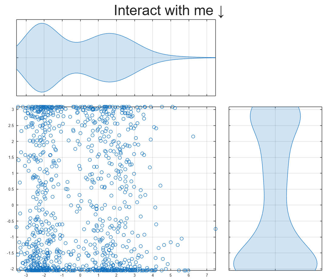
To learn about more Graphics and App Building features in R2026a, check out today's blog article:
I submitted a Matlab support case but posting this publicly to hopefully save people some trouble and see if anyone has ideas.
After upgrading my workstation from Ubuntu 25.10 to Ubuntu 26.04 LTS, MATLAB GUI consistently prints this terminal error on shutdown:
free(): chunks in smallbin corrupted
MATLAB appears to run normally, but closing the GUI takes a long time and sometimes produces crash dumps. The terminal error occurs every time I close the GUI, but crash dumps are intermittent. I attached one R2026a crash dump. I had zero issues on Ubuntu 25.10.
Affected versions:
- MATLAB R2026a
- MATLAB R2025b
- I suspect any 'new desktop' version
System:
- Ubuntu 26.04 LTS
- AMD EPYC 7443P
- NVIDIA RTX 3090
- Ubuntu 26.04 default NVIDIA driver: nvidia-driver-595-open, 595.58.03
- NVIDIA module path: /lib/modules/7.0.0-14-generic/kernel/nvidia-595-open/nvidia.ko
- glibc 2.43
Important note: the error first occurred with a clean MathWorks MATLAB installation before installing the Ubuntu/Debian `matlab-support` package. I later tested after installing `matlab-support`, which I understand modifies/renames some MATLAB-bundled libraries so MATLAB uses selected system libraries instead. The same shutdown error occurs both before and after applying `matlab-support`. This suggests the issue is not caused solely by the Debian/Ubuntu `matlab-support` integration or solely by one of the libraries it substitutes.
The attached crash dump shows abort/free() heap corruption detected in libc, but the higher-level stack includes MATLAB libraries such as:
- libmwcppmicroservices.so
- libmwmodule_descriptor_implementation.so
- libmwmatlab_main_lib.so
- libmwfoundation_threadpool.so
The issue appears GUI-specific. Using these startup flags shut down cleanly:
- matlab -batch
- matlab -nodesktop
- matlab -nodisplay
The shutdown error still occurs with these startup flags:
- normal GUI launch
- -nosplash
- -nojvm
- -softwareopengl
- -cefdisablegpu
The issue also persists after:
- renaming/resetting ~/.matlab/R2026a and ~/.MathWorks/R2026a
- launching with a clean environment without LD_LIBRARY_PATH, LD_PRELOAD, MATLAB_JAVA, JAVA_HOME, JRE_HOME, etc.
- testing a new Ubuntu user account
- testing Ubuntu/GNOME, GNOME, and Xfce X11 sessions
- testing NO_AT_BRIDGE=1 and GTK_USE_PORTAL=0
- temporarily moving ~/.MathWorks/ServiceHost
- testing GLIBC_TUNABLES=glibc.malloc.tcache_count=0
- trying to capture a system coredump with ulimit -c unlimited / coredumpctl; no system coredump was produced
Because R2025b and R2026a are both affected, terminal-only modes exit cleanly, the problem occurs across GNOME/Wayland and Xfce/X11, and the error occurred on a clean MATLAB install before any `matlab-support` modifications, this appears related to MATLAB GUI shutdown on Ubuntu 26.04 / glibc 2.43 rather than a corrupted MATLAB preference folder, a single desktop session, or the Ubuntu `matlab-support` package.
Example crash dump:
Hi everyone
My blog post about the latest MATLAB release was published yesterday MATLAB R2026a has been released – What’s new? » The MATLAB Blog - MATLAB & Simulink
There are a lot of new features and performance enhancements and from conversations I've had across several social media platforms., it seems that the new metafunction functionality is emerging as a user favourite. What are you most excited to see?
Cheers,
Mike
Do we know if MATLAB is being used on the Artemis II (moon mission) spacecraft itself? Like is the crew running MATLAB programs? I imagine it was probably at least used in development of some of the components of the spacecraft, rockets, or launch building. Or is it used for any of the image analysis of the images collected by the spacecraft?
MATLAB interprets the first block of uninterupted comments in a function file as documentation. Consider a simple example.
% myfunc This is my function
%
% See also sin
function z = myfunc(x, y)
z = x + y;
end
Those comments are printed in the command window with "help myfunc" and displayed in a separate window with "doc myfunc". A lot of useful things happen behind the scenes as well.
- Hyperlinks are automatically added for valid file names after "See also".
- When dealing with classes, the doc command automatically appends the comment block with a lists of properties and methods.
All this is very handy and as been around for quite some time. However, the doc browser isn't great (forward/back feature was removed several versons ago), the text formatting isn't great, and there is no way to display math.
Although pretty text/math can be displayed in a live document, the traditional *.mlx file format does not always play nice with Git and I have avoided them. However, live documents can now (since 2025a?) be saved in a pure text format, so I began to wonder if all functions should be written in this style. Turns out that all you have to do is append these lines:
%[appendix]{"version":"1.0"}
%---
to the end of any function file to make it a live function. Doing so changes how MATLAB manages that first comment block. The help command seems to be unaffacted, although [text] may appear at the start of each comment line (depending on if the file was create as a live function or subsequently converted). The doc command behaves very different: instead of bringing up the traditional window for custom documentation, the comment block looks like it gets published to HTML and looks more similar to standard MATLAB help. This is a win in some ways, but the "See also" capabilitity is lost.
Curiously, the same text can be appended to the end of a class definition file with some affect. It does not change how the file shows up in the editor, but as in live functions, comments are published when using the doc command. So we are partway to something like a "live class", but not quite.
Should one stick with traditional *.m files or make everything live? Neither does a great job for functions/classes in a namespace--references must explicitly know absolute location in traditional functions, and there is no "See also" concept in a live function. Do we need a command, like cdoc (custom documentation), that pulls out the comment block, publishing formatted text to HTML while simultaneously resolving "See also" references as hyperlinks? If so, it would be great if there were other special commands like "See examples" that would automatically copy and then open an example script for the end user.
Hi all,
I'm a UX researcher here at MathWorks working on the MathWorks Central Community. We're testing a new feature to make it easier to ask a question, and we'd love to hear from community members like you.
Sessions will be next week. They are remote, up to 2 hours (often shorter), and participants receive a $100 stipend. If you're interested, you can click here to schedule.
Thanks in advance! Your feedback directly shapes what gets built.
--David, MathWorks UX Research
Hello Community,
Registration is now open for the MathWorks Automotive Conference 2026 North America. Join industry leaders and MathWorks experts to learn about the latest trends in:
- Software-defined vehicles
- Generative AI
- Virtual vehicles
- AI and machine learning
Event details
- Date: April 28, 2026
- Location: Saint John’s Resort, Plymouth, MI
This conference is a great opportunity to connect with MathWorks and industry peers—and to explore what’s next in automotive engineering. We encourage you to register today.
We hope to see you there.
Absolutely!
65%
Probably
8%
Sometimes yes, sometimes no
8%
Unlikely
15%
Never!
4%
26 个投票
Matlab seems to follow a rule that iterative reduction operators give appropriate non-empty values to empty inputs. Examples include,
sum([])
prod([])
all([])
any([])
Is it an oversight not to do something similar for min and max?
max([])
For non-empty A and B,
max([A,B])= max(max(A), max(B))
The extension to B=[] should therefore satisfy,
max(A)=max(max(A),max([]))
for any A, which will only be true if we define max([])=-inf.
The 550,000th question has been asked on Answers.
Have you ever wondered what it takes to send live audio from one computer to another? While we use apps like Discord and Zoom every day, the core technology behind real-time voice communication is a fascinating blend of audio processing and networking. Building a simple walkie-talkie is a perfect project for demystifying these concepts, and you can do it all within the powerful environment of MATLAB.
This article will guide you through creating a functional, real-time, push-to-talk walkie-talkie. We won't be building a replacement for a commercial radio, but we will create a powerful educational tool that demonstrates the fundamentals of digital signal processing and network communication.
The Purpose: Why Build This?
The goal isn't just to talk to a colleague across the office; it's to learn by doing. By building this project, you will:
Understand Audio I/O: Learn how MATLAB interacts with your computer’s microphone and speakers.
Grasp Network Communication: See how to send data packets over a local network using the UDP protocol.
Solve Real-Time Challenges: Confront and solve issues like latency, choppy audio, and continuous data streaming.
The Core Components
Our walkie-talkie will consist of two main scripts:
Sender.m: This script will run on the transmitting computer. It listens to the microphone when a key is pressed, sending the audio data in small chunks over the network.
Receiver.m: This script runs on the receiving computer. It continuously listens for incoming data packets and plays them through the speakers as they arrive.
Step 1: Getting Audio In and Out
Before we touch networking, let's make sure we can capture and play audio. MATLAB's built-in audiorecorder and audioplayer objects make this simple.
Problem Encountered: How do you even access the microphone?
Solution: The audiorecorder object gives us straightforward control.
code
% --- Test Audio Capture and Playback ---
Fs = 8000; % Sample rate in Hz
nBits = 16; % Number of bits per sample
nChannels = 1; % Mono audio
% Create a recorder object
recObj = audiorecorder(Fs, nBits, nChannels);
disp('Start speaking for 3 seconds.');
recordblocking(recObj, 3); % Record for 3 seconds
disp('End of Recording.');
% Get the audio data
audioData = getaudiodata(recObj);
% Play it back
playObj = audioplayer(audioData, Fs);
play(playObj);
Running this script confirms that your microphone and speakers are correctly configured and accessible by MATLAB.
Step 2: Sending Voice Over the Network
Now, we need to send the audioData to another computer. For real-time applications like this, the UDP (User Datagram Protocol) is the ideal choice. It’s a "fire-and-forget" protocol that prioritizes speed over perfect reliability. Losing a tiny packet of audio is better than waiting for it to be re-sent, which would cause noticeable delays (latency).
Problem Encountered: How do you send data continuously without overwhelming the network or the receiver?
Solution: We'll send the audio in small, manageable chunks inside a loop. We need to create a UDP Port object to handle the communication.
Here's the basic structure for the Sender.m script:
code
% --- Sender.m ---
% Define network parameters
remoteIP = '192.168.1.101'; % <--- CHANGE THIS to the receiver's IP
remotePort = 3000;
localPort = 3001;
% Create UDP Port object
udpSender = udpport("LocalPort", localPort, "EnablePortSharing", true);
% Configure audio recorder
Fs = 8000;
nBits = 16;
nChannels = 1;
recObj = audiorecorder(Fs, nBits, nChannels);
disp('Press any key to start transmitting. Press Ctrl+C to stop.');
pause; % Wait for user to press a key
% Start the Push-to-Talk loop
disp('Transmitting... (Hold Ctrl+C to exit)');
while true
recordblocking(recObj, 0.1); % Record a 0.1-second chunk
audioChunk = getaudiodata(recObj);
% Send the audio chunk over UDP
write(udpSender, audioChunk, "double", remoteIP, remotePort);
end
And here is the corresponding Receiver.m script:
code
Matlab
% --- Receiver.m ---
% Define network parameters
localPort = 3000;
% Create UDP Port object
udpReceiver = udpport("LocalPort", localPort, "EnablePortSharing", true, "Timeout", 30);
% Configure audio player
Fs = 8000;
playerObj = audioplayer(zeros(Fs*0.1, 1), Fs); % Pre-buffer
disp('Listening for incoming audio...');
% Start the listening loop
while true
% Wait for and receive data
[audioChunk, ~, ~] = read(udpReceiver, Fs*0.1, "double");
if ~isempty(audioChunk)
% Play the received audio chunk
play(playerObj, audioChunk);
else
disp('No data received. Still listening...');
end
end
Step 3: Solving Real-World Hurdles
Running the code above might work, but you'll quickly notice some issues.
Problem 1: Choppy Audio and High Latency
The audio might sound robotic or delayed. This is because of the buffer size and the processing time. Sending tiny chunks frequently can cause overhead, while sending large chunks causes delay.
Solution: The key is to find a balance.
Tune the Chunk Size: The 0.1 second chunk size in the sender (recordblocking(recObj, 0.1)) is a good starting point. Experiment with values between 0.05 and 0.2. Smaller values reduce latency but increase network traffic.
Use a Buffered Player: Instead of creating a new audioplayer for every chunk, we create one at the start and feed it new data. Our receiver code already does this, which is more efficient.
Problem 2: No Real "Push-to-Talk"
Our sender script starts transmitting and doesn't stop. A real walkie-talkie only transmits when a button is held down.
Solution: Simulating this in a script requires a more advanced technique, ideally using a MATLAB App Designer GUI. However, we can create a simple command-window version using a figure's KeyPressFcn.
Here is an improved concept for the Sender that simulates radio push-to-talk, e.g. https://www.retevis.com/blog/ptt-push-to-talk-walkie-talkies-guide
% --- Advanced_Sender.m ---
function PushToTalkSender()
% -- Configuration --
remoteIP = '192.168.1.101'; % <--- CHANGE THIS
remotePort = 3000;
localPort = 3001;
Fs = 8000;
% -- Setup --
udpSender = udpport("LocalPort", localPort);
recObj = audiorecorder(Fs, 16, 1);
% -- GUI for key press detection --
fig = uifigure('Name', 'Push-to-Talk (Hold ''t'')', 'Position', [100 100 300 100]);
fig.KeyPressFcn = @KeyPress;
fig.KeyReleaseFcn = @KeyRelease;
isTransmitting = false; % Flag to control transmission
disp('Focus on the figure window. Hold the ''t'' key to transmit.');
% --- Main Loop ---
while ishandle(fig)
if isTransmitting
% Non-blocking record and send would be ideal,
% but for simplicity we use short blocking chunks.
recordblocking(recObj, 0.1);
audioChunk = getaudiodata(recObj);
write(udpSender, audioChunk, "double", remoteIP, remotePort);
disp('Transmitting...');
else
pause(0.1); % Don't burn CPU when idle
end
drawnow; % Update figure window
end
% --- Callback Functions ---
function KeyPress(~, event)
if strcmp(event.Key, 't')
isTransmitting = true;
end
end
function KeyRelease(~, event)
if strcmp(event.Key, 't')
isTransmitting = false;
disp('Transmission stopped.');
end
end
end
Conclusion and Next Steps
You've now built the foundation of a real-time voice communication tool in MATLAB! You've learned how to capture audio, send it over a network using UDP, and handle some of the fundamental challenges of real-time streaming.
This project is the perfect starting point for more advanced explorations:
Build a Full GUI: Use App Designer to create a user-friendly interface with a proper push-to-talk radio button.
Implement Noise Reduction: Apply a filter (e.g., a simple low-pass or a more advanced spectral subtraction algorithm) to the audioChunk before sending it.
Add Channels: Modify the code to use different UDP ports, allowing users to select a "channel" to talk on.
In a previous discussion,
we looked at a variety of infallible tests for primality, but all of them were too slow to be viable for large numbers. In fact, all of the methods discussed there will fail miserably for even moderately large numbers, those with just a few dozen decimal digits. That does not even begin to push into the realm of large numbers. In turn, that forces us into a different realm of tests - tests which are usually and even almost always correct, but can sometimes incorrectly predict primality.
In this discussion, I will be trying to convince you that the Fermat test for primality can be a quite good test when the number is sufficiently large. Except of course, when it is really bad. Even so, the Fermat test for primality is both a useful tool as well as a necessary underpinning for several other better tests.
The Fermat test for primality relies on Fermat's little theorem, a perhaps under-appreciated tool. Even the name implies it is of little interest. I'm not taking about the famous last theorem, only proven in recent years, but his little theorem.
If you want to look over some nice ways to prove the little theorem, take a read in this link:
I will readily admit that long ago, when I learned about the little theorem in a nearly forgotten class, I thought it was interesting, but why would I care? Not until I learned more mathematics and saw Fermat’s little theorem appearing in different places did I begin to appreciate it. Fermat tells us that, IF P is a prime, AND w is co-prime with P (so the two are relatively prime, sharing no common factors except 1), then it must be true that
mod(w^(P-1),P) == 1
Try it out. Does it work? Be careful though as too large of an exponent will cause problems in double precision, and that is not difficult to do. As a test case that will not overwhelm doubles, note that 13 is prime, and 3 shares no common factors with 13, so we satisfy the requirements for Fermat's little theorem.
mod(3^12,13)
We can even verify that any co-prime of 13 will yield the same result.
mod((1:12).^12,13)
Indeed it worked, suggesting what we knew all along, that 13 is prime. The little Fermat test for primality of the number P uses a converse form of Fermat's little theorem, thus given a co-prime number w known as the witness, is that if
mod(w^(P-1),P)==1
then we have evidence that P is indeed prime. This is not conclusive evidence, but still it is evidence. It is not conclusive because the converse of a true statement is not always true.
The analogy I like here is if we lived in a universe where all crows are black. (I'll ask you to pretend this is true. In fact, some crows have a mutation, making them essentially albino crows. For the purposes of this thought experiment, pretend this cannot happen.) Now, suppose I show you a picture of a bird which happens to be black. Do you know the bird to be a crow? Of course not, as the bird may be a raven, or a redwing blackbird (until you see the splash of red on the wing), a common grackle, a European starling in summer plumage, a condor, etc. But having seen black plumage, it is now more likely the bird is indeed a crow. I would call this a moderately weak evidentiary test for crow-ness.
Little Fermat may seem to be of little value when testing for primality for two reasons. First, computing the remainder would seem to be highly CPU intensive for large P. In the example above, I had only to compute 3^12=531441, which is not that large. But for numbers with many thousands or millions of digits, directly raising even a number as small as 2 to that power will overwhelm any computer. Secondly, if we do that computation, little Fermat does not conclusively prove P to be prime.
Our savior in one respect is the powermod tool. And that helps greatly, since we can compute the remainder in a reasonable time. A powermod call is quite fast even for huge powers. (I won't get into how powermod works here, since that alone is probably worth a discussion. I could though, if I see some interest because there are some very pretty variations of the powermod algorithm. I hope to show you one of them when I discuss the Fibonacci test for primality in a future post.) Trying the little Fermat test using powermod on a number with 1207 decimal digits, I’ll first do a time check.
P = 4000*sym(2)^3999 - 1;
timeit(@() powermod(2,P-1,P))
As you can see, powermod really is pretty fast. Compared to an isprime test on that number it would show a significant difference.
I have said before that little Fermat is not a conclusive test. In fact, a good trick is to perform a second little Fermat test, using a different witness. If the second test also indicates primality, then we have additional evidence that P is in fact prime.
w = [2 3]; % Two parallel witnesses
powermod(w,P-1,P)
This value for P is indeed prime, and little Fermat suggests it is, doubly suggestive in that test since I actually performed two parallel tests. Here however, we need to understand when it will fail, and how often it will fail.
If we perform a little Fermat test for primality, we will never see false negatives, that is, if any test with any witness ever indicates a number is composite, then it is certainly composite. (The contrapositive of a true statement is always true.) The alternate class of failure is the false positive, where little Fermat indicates a number is prime when it was actually composite.
If P is composite, and w co-prime with P, we call P a Fermat pseudo-prime for the witness w if we see a remainder of 1 when P was in fact composite. When that happens, the witness (w) is called a Fermat liar for the primality of P. (A list of some Fermat pseudo-primes where 2 is a Fermat liar can be found in sequence A001567 of the OEIS.)
In the case of 4000*2^3999-1, I claimed the number to be in fact prime, and it was identified so (as PROBABLY prime by little Fermat. Next, consider another number from that same family. I’ll perform three parallel tests on it, with witnesses 2, 3, and 5. This will suggest the value of doing parallel tests on a number to reduce the failure rate from little Fermat.
P2 = 1024*sym(2)^1023 - 1;
w = [2; 3; 5];
gcd(w,P2)
F2 = powermod(w,P2-1,P2)
logical(F2 == 1)
As you can see, P2 is co-prime with all of 2, 3 and 5, but 2 is a Fermat liar, whilst 3 and 5 are Fermat truth tellers, identifying P2 as certainly composite. So the little Fermat test can definitely fail for SOME witnesses, since we see a disagreement. However, an interesting fact about P2 above is it is also a Mersenne number with prime exponent, thus it can be written as 2^1033-1, where 1033 is prime. I can go into more detail about this case later, but we can show that 2 is always a Fermat liar for composite Mersenne numbers when the exponent is itself prime. I’ll try to leave more detail on this matter in a future discussion, or perhaps a comment.
Next, consider the composite integer 51=3*17. As the product of two primes, it is clearly not itself prime.
P51 = 51;
w0 = 2:P51-2;
w = w0(gcd(w0,P51) == 1)
Note that I did not include 1 or 50 in that set, since 1 raised to any power is 1, and 50 is congruent to -1, mod 51. -1 raised to any even power is also always 1, and 51-1 is an even number. And so when we are working modulo 51, both 1 and 50 are not useful witnesses in terms of the little Fermat test.
R = powermod(w,P-1,P)
w(R == 1)
This teaches us that when 51 is tested for primality using the little Fermat test, there are 2 distinct witnesses w (16 and 35) we could have chosen which would have been Fermat liars, but all 28 other potential co-prime witnesses would have been truth tellers, accurately showing 51 to be composite. Proportionally, little Fermat will have been correct roughly 93% of the time, since only 2 of these 30 possible tests returned a false positive. (I’ll add that for any modulus P, if w<P is not co-prime with the modulus, then the computation mod(w^(P-1),P) will always return a non-unit result, and therefore we can theoretically use any integer w from the set 2:P-2 as a witness. However if w is co-prime with P then P is clearly not prime, and the entire problem becomes a little less interesting. As such, I will only consider co-prime witnesses for this discussion.) Regardless, that would make the little Fermat test for P=51 even more often correct, since it returns the correct result of composite for 46 out of the 48 possible witnesses 2:49. Does this mean Little Fermat is indeed the basis for a good test to rely on to learn if a number is prime? Well, yes. And no.
Little Fermat forms a very good test most of the time, but reliance is a strong word. This means we need to explore the little Fermat test in more depth, focusing on Fermat liars and the case of false positives. To offer some appreciation of the false positive rate, offline, I have tested all composite integers between 4 and 10000, for all their possible co-prime witnesses.
load FermatLiarsData
In that .mat file, I've saved three vectors, X, witnessCount, and liarCount. X is there just to use for plotting purposes and is NaN for all non-composite entries.
whos X witnessCount liarCount
The vector witnessCount is the number of valid witnesses for the corresponding number in X. Corresponding to that is the vector liarCount, which is the number of Fermat liars I found for each composite in X.
How many Fermat test useful witnesses are there for any integer X? This is just 2 less than the number of coprimes of X. The number of coprimes is given by the Euler totient function, commonly called phi(X). (I’ll be going into more depth on the totient in the next chapter of this series, because the Euler totient is a crucial part of understanding how all of this works.)
The witness count is phi(X)-2. Why subtract 2? 1 can never be a witness, but 1 is technically coprime to everything. The same applies to X-1 (which is congruent to -1 mod X.) As such, there are phi(X)-2 coprimes to consider. (I've posted a function called totient on the FEX, but it is easily computed if you know the factorization of X. Or for small numbers, you can just use GCD to identify all co-primes, and count them.)
plot(X,witnessCount,'.')
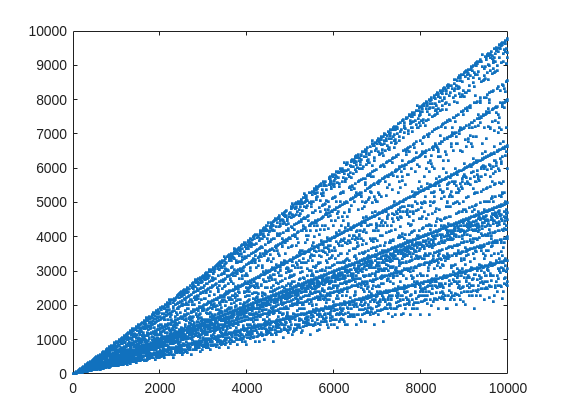
From that plot, you can learn a few interesting things. (As a mathematician, this is what I love the most, thus to look at whay may be the simplest, most boring plot, and try to find something of value, something I had never thought of before.) For example, we know that when X is prime, then everything from the set 2:X-2 is a valid witness. So the upper boundary on that plot will be the line y==x. As well, there are a few numbers where the order of the set of witnesses will be close to the maximum possible. For example, 961=31*31, has 928 valid witnesses. That makes some sense, as 961 is the square of a prime (31), so we know 961 is divisible only by 31. Only multiples of 31 will not be coprime with 961.
But how about the lower boundary? The least number of valid witnesses will always come from highly composite numbers, because they will share common factors with almost everything. For example 30 = 2*3*5, or 210=2*3*5*7.
witnessCount([30 210 420])
A good discussion about the lower bound for that plot can be found here:
What really matters to us though, is the fraction of the useful witnesses for a little Fermat test that yield a false positive.
plot(X,liarCount./witnessCount,'b.')
Cind = liarCount == witnessCount;
hold on
plot(X(Cind),1,'ro')
ylabel('Liar fraction')
xlabel('X')
title('Fermat pseudo-prime strength')
hold off
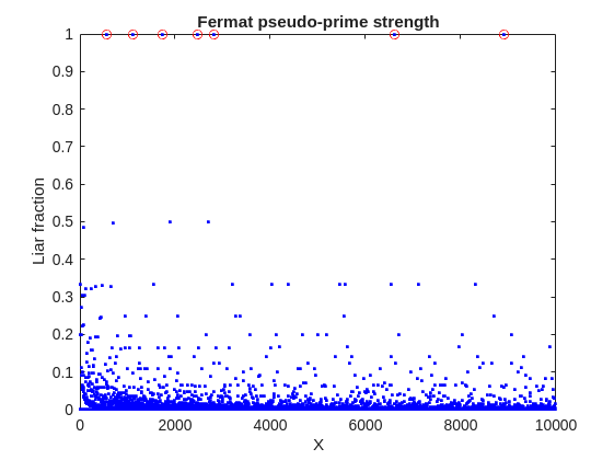
A look at this plot shows seven circles in red, corresponding to X from the list {561, 1105, 1729, 2465, 2821, 6601, 8911} which are collectively known as Carmichael numbers. These are numbers where all witnesses return a false positive. Carmichael numbers are themselves fairly rare. You can find a list of them as sequence A002997 in the OEIS. And for those of you who have never wandered around the OEIS, please take this opportunity to do so now. The OEIS stands for Online Encyclopedia of Integer Sequences. It contains a wealth of interesting knowledge about integers and integer sequences.)
There are a few other interesting numbers we can find in that plot, like 91 and 703, where roughly 50% of the valid witnesses yield false positives. Of the complete set, which numbers did return at least a 25% false positive rate for primality? These numbers would be known as strong pseudo-primes for the little Fermat test, because they are pseudo-primes for at least 25% of the potential witnesses. These strong pseudo-primes have some interesting similarities to the Carmichael numbers. (My next post will go into more depth on Carmichael numbers and strong pseudo-primes. At the moment, I am merely interested in looking at the how often the little Fermat test fails overall.)
find(liarCount./witnessCount> 0.25)
You should notice the spacing between successive strong Fermat pseudo-primes is growing slowly, with a spacing of roughly 800 on average in the vicinity of 10000. If I step out beyond by a factor of 10, the next strong Fermat pseudo-primes after 1e5 are {101101, 104653, 107185, 109061, 111361, 114589, 115921 126217, 126673}, so that average spacing is definitely growing.
Given that set, now we can look at the prime factorizations of each of those strong pseudo-primes. Can we learn something about them?
arrayfun(@factor,find(liarCount./witnessCount> 0.25),'UniformOutput',false)
Perhaps the most glaring thing I see in that set of factors is almost all of those strong Fermat pseudo-primes are square free. That is, in that list, only 45=3*3*5 had any replicated factor at all. That property of being square free is something we will see is necessary to be a Carmichael number, but it also suggests that a simple roughness test applied in advance would have eliminated almost all of those strong pseudo-primes as obviously not prime, even at a very low level of roughness.
In fact, for most composite integers, most witnesses do indeed return a negative, indicating the number is not prime, and therefore composite. Little Fermat does not commonly tell falsehoods, even though it can do so.
semilogy(X,movmedian(liarCount./witnessCount,20,'omitnan'),'b-')
title('False positive fraction for composites')
yline(0.0003,'r')

We can learn from this last plot that as the number to be tested grows large, the median false positive rate for little Fermat, even for X as low as only 10000, is roughly 0.0003. (It continues to decrease for larger X too. In fact, I’ve read that when X is on the order of 2^256, the relative fraction of Fermat liars is on the order of 1 in 1e12, and it continues to decrease as X grows in magnitude. In my eyes, that seems pretty good for an imperfect test. Not perfect, but not bad when paired with roughness and perhaps a second little Fermat test using a different witness, and we will start to see tests which bear a higher degree of strength.)
I’ll stop at this point in this post because the post is getting lengthy. In my next post, I’d like to visit some questions about what are Carmichael numbers, about whether some witnesses are better than others, and if there are any numbers which lack any Fermat liars. However, in order to dive more deeply, I will need to explain how/why/when the little Fermat test works, and what causes Fermat liars. Stay tuned, because this starts to get interesting.
If you have published add-ons on File Exchange, you may have noticed that we recently added a new, unique package name field to all add-ons. This enables future support for automated installation with the MATLAB Package Manager. This name will be a unique identifier for your add-on and does not affect the existing add-on title, any file names, or the URL of your add-on.
📝 Update and review until April 10
We generated default package names for all add-ons. You can review and update the package name for your add-ons until April 10, 2026. Review your package names now:
After April 10, you will need to create a new version to change your package name.
🚀 More changes coming with the MATLAB R2026b prerelease
Starting with the MATLAB R2026b prerelease, these package names will take effect. At that time, the package name may appear on the File Exchange page for your add-on.
Keep your eyes peeled for exciting changes coming soon to your add-ons on File Exchange!
Cantera is an open-source suite of tools for problems involving chemical kinetics, thermodynamics, and transport processes. Dr. Su Sun, a recent graduate from Northeastern Chemical Engineering Ph.D. program made significant contributions to MATLAB interface for Cantera in Cantera Release 3.2.0 in collaboration with Dr. Richard West, other Cantera developers, and MathWorks Advanced Support and Development Teams. As part of this Release, MATLAB interface for Cantera transitioned to using the new MATLAB- C++ interface and expanded their unit testing. Further information is available here.
I began coding in MATLAB less than 2 months ago for a class at community college. Alongside the course content, I also completed the MATLAB onramp and introduction to linear algebra self-paced online courses. I think this is the most fun I've had coding since back when I used to make Scratch projects in elementary school. I'm kind of curious if I could recreate some of my favorite childhood Scratch games here.
Anyways, I just wanted to introduce myself since I plan to be really active this year. My name is Mehreen (meh like the meh emoji from the Emoji movie, reen like screen), I'm a data science undergrad sophomore from the U.S. and it's nice to meet you!
An emirp is a prime that is prime when viewed in in both directions. They are not too difficult to find at a lower level. For example...
isprime([199 991])
Gosh, that was easy. But what happens if the number is a bit larger? The problem is, primes themselves tend to be rare on the number line when you get into thousands or tens of thousands of decimal digits. And recently, I read that a world record size prime had been found in this form. You have probably all heard of Matt Parker and numberphile.
And so, I decided that MATLAB would be capable of doing better. Why not? After all, at the time, the record size emirp had only 10002 decimal digits.
How would I solve this problem? First, we can very simply write a potential emirp as
10^n + a
then we can form the flipped version as
ahat*10^(n-d) + 1
where ahat is the decimally flipped version of a, and d is chosen based on the number of decimal digits in the number a itself. Not all emirps will be of that form of course, but using all of those powers of 10 makes it easy to construct a large number and its reversed form. And that is a huge benefit in this. For example,
Pfor = sym(10)^101 + 943
Prev = 349*sym(10)^99 + 1
It is easier to view these numbers using a little code I wrote, one that redacts most of those boring zeros.
emirpdisplay(Pfor)
emirpdisplay(Prev)
And yes, they are both prime, and they both have 102 decimal digits.
isprime([Pfor,Prev])
Sadly, even numbers that large are very small potatoes, at least in the world of large primes. So how do we solve for a much larger prime pair using MATLAB?
The first thing I want to do is to employ roughness at a high level. If a number is prime, then it is maximally rough. (I posted a few discussions about roughness some time ago.)
https://www.mathworks.com/matlabcentral/discussions/tips/879745-primes-and-rough-numbers-basic-ideas
In this case, I'm going to look for serious roughness, thus 2e9-rough numbers. Again, a number is k-rough if its smallest prime factor is greater than k. There are roughly 98 million primes below 2e9.
The general idea is to compute the remainders of 10^12345, modulo every prime in that set of primes below 2e9. This MUST be done using int64 or uint64 arithmetic, as doubles will start to fail you above
format short g
sqrt(flintmax)
The sqrt is in there because we will be multiplying numbers together here, and we need always to stay below intmax for the integer format you are working with. However, if we work in an integer format, we can get as high as 2e9 easily enough, by going to int64 or uint64.
sqrt(double(intmax('int64')))
And, yes, this means I could have gone as high as primes(3e9), however, I stopped at 2e9 due to the amount of RAM on my computer. 98 million primes seemed enough for this task. And even then, I found myself working with all of the cores on my computer. (Note that I found int64 arithmetic will only fire up the performance cores on your Mac via automatic multi-threading. Mine has 12 performance cores, even though it has 16 total cores.)
I computed the remainders of 10^12345 with respect to each prime in that set using a variation of the powermod algorithm. (Not powermod itself, which was itself not sufficiently fast for my purposes.) Once I had those 98 millin remainders in a vector, then it became easy to use a variation of the sieve of Eratosthenes to identify 2e9-rough numbers.
For example, working at 101 decimal digits, if I search for primes of the form 10^101+a, with a in the interval [1,10000], there are 256 numbers of that form which are 2e9-rough. Roughness is a HUGE benefit, since as you can see here, I would not want to test for primality all 10000 possible integers from that interval.
Next, I flip those 256 rough numbers into their mirror image form. Which members of that set are also rough in the mirror image form? We would then see this further reduces the set to only 34 candidates we need test for primality which were rough in both directions. With now only a few direct tests for primality, we would find that pair of 102 digit primes shown above.
Of course, I'm still needing to work with primes in the regime of 10000 plus decimal digits, and that means I need to be smarter about how I test a number to be prime. The isprime test given by sym/isprime only survives out to around 1000 decimal digits before it starts to get too slow. That means I need to perform Fermat tests to screen numbers for primality. If that indicates potential primality, I currently use a Miller-Rabin code to verify that result, one based on the tool Java.Math.BigInteger.isProbablePrime.
And since Wikipedia tells me the current world record known emirp was
117,954,861 * 10^11111 + 1 discovered by Mykola Kamenyuk
that tells me I need to look further out yet. I chose an exponent of 12345, so starting at 10^12345. Last night I set my Mac to work, with all cores a-fumbling, a-rumbling at the task as I slept. Around 4 am this morning, it found this number:
emirp = @(N,a) sym(10)^N + a;
Pfor = emirp(12345,10519197);
Prev = sym(flip(char(Pfor)));
emirpdisplay(Pfor)
emirpdisplay(Prev)
isProbablePrimeFLT([Pfor,Prev],210)
I'm afraid you will need to take my word for it that both also satisfy a more robust test of primality, as even a Miller-Rabin test that will take more time than the MATLAB version we get for use in a discussion will allow. As far as a better test in the form of the MATLAB isprime utility to verify true primality, that test is still running on my computer. I'll check back in a few hours to see if it fininshed.
Anyway, the above numbers now form the new world record known emirp pair, at 12346 decimal digits. Yes, I do recognize this is still what I would call low hanging fruit, that having announced a largest prime of this form, someone else willl find one yet larger in a few weeks or months. But even so, for the moment, MATLAB owns the world record!
If anyone else wants a version of the codes I used for the search, I've attached a version (emirpsearchpar.m) that employs the parallel processing toolbox. I do have as well a serial version which is of course, much, much slower. It would be fun to crowd source a larger world record yet from the MATLAB community.