搜索
t = turtle(); % Start a turtle
t.forward(100); % Move forward by 100
t.backward(100); % Move backward by 100
t.left(90); % Turn left by 90 degrees
t.right(90); % Tur right by 90 degrees
t.goto(100, 100); % Move to (100, 100)
t.turnto(90); % Turn to 90 degrees, i.e. north
t.speed(1000); % Set turtle speed as 1000 (default: 500)
t.pen_up(); % Pen up. Turtle leaves no trace.
t.pen_down(); % Pen down. Turtle leaves a trace again.
t.color('b'); % Change line color to 'b'
t.begin_fill(FaceColor, EdgeColor, FaceAlpha); % Start filling
t.end_fill(); % End filling
t.change_icon('person.png'); % Change the icon to 'person.png'
t.clear(); % Clear the Axes
classdef turtle < handle
properties (GetAccess = public, SetAccess = private)
x = 0
y = 0
q = 0
end
properties (SetAccess = public)
speed (1, 1) double = 500
end
properties (GetAccess = private)
speed_reg = 100
n_steps = 20
ax
l
ht
im
is_pen_up = false
is_filling = false
fill_color
fill_alpha
end
methods
function obj = turtle()
figure(Name='MATurtle', NumberTitle='off')
obj.ax = axes(box="on");
hold on,
obj.ht = hgtransform();
icon = flipud(imread('turtle.png'));
obj.im = imagesc(obj.ht, icon, ...
XData=[-30, 30], YData=[-30, 30], ...
AlphaData=(255 - double(rgb2gray(icon)))/255);
obj.l = plot(obj.x, obj.y, 'k');
obj.ax.XLim = [-500, 500];
obj.ax.YLim = [-500, 500];
obj.ax.DataAspectRatio = [1, 1, 1];
obj.ax.Toolbar.Visible = 'off';
disableDefaultInteractivity(obj.ax);
end
function home(obj)
obj.x = 0;
obj.y = 0;
obj.ht.Matrix = eye(4);
end
function forward(obj, dist)
obj.step(dist);
end
function backward(obj, dist)
obj.step(-dist)
end
function step(obj, delta)
if numel(delta) == 1
delta = delta*[cosd(obj.q), sind(obj.q)];
end
if obj.is_filling
obj.fill(delta);
else
obj.move(delta);
end
end
function goto(obj, x, y)
dx = x - obj.x;
dy = y - obj.y;
obj.turnto(rad2deg(atan2(dy, dx)));
obj.step([dx, dy]);
end
function left(obj, q)
obj.turn(q);
end
function right(obj, q)
obj.turn(-q);
end
function turnto(obj, q)
obj.turn(obj.wrap_angle(q - obj.q, -180));
end
function pen_up(obj)
if obj.is_filling
warning('not available while filling')
return
end
obj.is_pen_up = true;
end
function pen_down(obj, go)
if obj.is_pen_up
if nargin == 1
obj.l(end+1) = plot(obj.x, obj.y, Color=obj.l(end).Color);
else
obj.l(end+1) = go;
end
uistack(obj.ht, 'top')
end
obj.is_pen_up = false;
end
function color(obj, line_color)
if obj.is_filling
warning('not available while filling')
return
end
obj.pen_up();
obj.pen_down(plot(obj.x, obj.y, Color=line_color));
end
function begin_fill(obj, FaceColor, EdgeColor, FaceAlpha)
arguments
obj
FaceColor = [.6, .9, .6];
EdgeColor = [0 0.4470 0.7410];
FaceAlpha = 1;
end
if obj.is_filling
warning('already filling')
return
end
obj.fill_color = FaceColor;
obj.fill_alpha = FaceAlpha;
obj.pen_up();
obj.pen_down(patch(obj.x, obj.y, [1, 1, 1], ...
EdgeColor=EdgeColor, FaceAlpha=0));
obj.is_filling = true;
end
function end_fill(obj)
if ~obj.is_filling
warning('not filling now')
return
end
obj.l(end).FaceColor = obj.fill_color;
obj.l(end).FaceAlpha = obj.fill_alpha;
obj.is_filling = false;
end
function change_icon(obj, filename)
icon = flipud(imread(filename));
obj.im.CData = icon;
obj.im.AlphaData = (255 - double(rgb2gray(icon)))/255;
end
function clear(obj)
obj.x = 0;
obj.y = 0;
delete(obj.ax.Children(2:end));
obj.l = plot(0, 0, 'k');
obj.ht.Matrix = eye(4);
end
end
methods (Access = private)
function animated_step(obj, delta, q, initFcn, updateFcn)
arguments
obj
delta
q
initFcn = @() []
updateFcn = @(~, ~) []
end
dx = delta(1)/obj.n_steps;
dy = delta(2)/obj.n_steps;
dq = q/obj.n_steps;
pause_duration = norm(delta)/obj.speed/obj.speed_reg;
initFcn();
for i = 1:obj.n_steps
updateFcn(dx, dy);
obj.ht.Matrix = makehgtform(...
translate=[obj.x + dx*i, obj.y + dy*i, 0], ...
zrotate=deg2rad(obj.q + dq*i));
pause(pause_duration)
drawnow limitrate
end
obj.x = obj.x + delta(1);
obj.y = obj.y + delta(2);
end
function obj = turn(obj, q)
obj.animated_step([0, 0], q);
obj.q = obj.wrap_angle(obj.q + q, 0);
end
function move(obj, delta)
initFcn = @() [];
updateFcn = @(dx, dy) [];
if ~obj.is_pen_up
initFcn = @() initializeLine();
updateFcn = @(dx, dy) obj.update_end_point(obj.l(end), dx, dy);
end
function initializeLine()
obj.l(end).XData(end+1) = obj.l(end).XData(end);
obj.l(end).YData(end+1) = obj.l(end).YData(end);
end
obj.animated_step(delta, 0, initFcn, updateFcn);
end
function obj = fill(obj, delta)
initFcn = @() initializePatch();
updateFcn = @(dx, dy) obj.update_end_point(obj.l(end), dx, dy);
function initializePatch()
obj.l(end).Vertices(end+1, :) = obj.l(end).Vertices(end, :);
obj.l(end).Faces = 1:size(obj.l(end).Vertices, 1);
end
obj.animated_step(delta, 0, initFcn, updateFcn);
end
end
methods (Static, Access = private)
function update_end_point(l, dx, dy)
l.XData(end) = l.XData(end) + dx;
l.YData(end) = l.YData(end) + dy;
end
function q = wrap_angle(q, min_angle)
q = mod(q - min_angle, 360) + min_angle;
end
end
end
I would like to zoom directly on the selected region when using  on my image created with image or imagesc. First of all, I would recommend using image or imagesc and not imshow for this case, see comparison here: Differences between imshow() and image()? However when zooming Stretch-to-Fill behavior happens and I don't want that. Try range zoom to image generated by this code:
fig = uifigure;
ax = uiaxes(fig);
im = imread("peppers.png");
h = imagesc(im,"Parent",ax);
axis(ax,'tight', 'off')
I can fix that with manualy setting data aspect ratio:
daspect(ax,[1 1 1])
However, I need this code to run automatically after zooming. So I create zoom object and ActionPostCallback which is called everytime after I zoom, see zoom - ActionPostCallback.
z = zoom(ax);
z.ActionPostCallback = @(fig,ax) daspect(ax.Axes,[1 1 1]);
If you need, you can also create ActionPreCallback which is called everytime before I zoom, see zoom - ActionPreCallback.
z.ActionPreCallback = @(fig,ax) daspect(ax.Axes,'auto');
Code written and run in R2025a.
I am thrilled python interoperability now seems to work for me with my APPLE M1 MacBookPro and MATLAB V2025a. The available instructions are still, shall we say, cryptic. Here is a summary of my interaction with GPT 4o to get this to work.
===========================================================
MATLAB R2025a + Python (Astropy) Integration on Apple Silicon (M1/M2/M3 Macs)
===========================================================
Author: D. Carlsmith, documented with ChatGPT
Last updated: July 2025
This guide provides full instructions, gotchas, and workarounds to run Python 3.10 with MATLAB R2025a (Apple Silicon/macOS) using native ARM64 Python and calling modules like Astropy, Numpy, etc. from within MATLAB.
===========================================================
Overview
===========================================================
- MATLAB R2025a on Apple Silicon (M1/M2/M3) runs as "maca64" (native ARM64).
- To call Python from MATLAB, the Python interpreter must match that architecture (ARM64).
- Using Intel Python (x86_64) with native MATLAB WILL NOT WORK.
- The cleanest solution: use Miniforge3 (Conda-forge's lightweight ARM64 distribution).
===========================================================
1. Install Miniforge3 (ARM64-native Conda)
===========================================================
In Terminal, run:
curl -LO https://github.com/conda-forge/miniforge/releases/latest/download/Miniforge3-MacOSX-arm64.sh
bash Miniforge3-MacOSX-arm64.sh
Follow prompts:
- Press ENTER to scroll through license.
- Type "yes" when asked to accept the license.
- Press ENTER to accept the default install location: ~/miniforge3
- When asked:
Do you wish to update your shell profile to automatically initialize conda? [yes|no]
Type: yes
===========================================================
2. Restart Terminal and Create a Python Environment for MATLAB
===========================================================
Run the following:
conda create -n matlab python=3.10 astropy numpy -y
conda activate matlab
Verify the Python path:
which python
Expected output:
/Users/YOURNAME/miniforge3/envs/matlab/bin/python
===========================================================
3. Verify Python + Astropy From Terminal
===========================================================
Run:
python -c "import astropy; print(astropy.__version__)"
Expected output:
6.x.x (or similar)
===========================================================
4. Configure MATLAB to Use This Python
===========================================================
In MATLAB R2025a (Apple Silicon):
clear classes
pyenv('Version', '/Users/YOURNAME/miniforge3/envs/matlab/bin/python')
py.sys.version
You should see the Python version printed (e.g. 3.10.18). No error means it's working.
===========================================================
5. Gotchas and Their Solutions
===========================================================
❌ Error: Python API functions are not available
→ Cause: Wrong architecture or broken .dylib
→ Fix: Use Miniforge ARM64 Python. DO NOT use Intel Anaconda.
❌ Error: Invalid text character (↑ points at __version__)
→ Cause: MATLAB can’t parse double underscores typed or pasted
→ Fix: Use: py.getattr(module, '__version__')
❌ Error: Unrecognized method 'separation' or 'sec'
→ Cause: MATLAB can't reflect dynamic Python methods
→ Fix: Use: py.getattr(obj, 'method')(args)
===========================================================
6. Run Full Verification in MATLAB
===========================================================
Paste this into MATLAB:
% Set environment
clear classes
pyenv('Version', '/Users/YOURNAME/miniforge3/envs/matlab/bin/python');
% Import modules
coords = py.importlib.import_module('astropy.coordinates');
time_mod = py.importlib.import_module('astropy.time');
table_mod = py.importlib.import_module('astropy.table');
% Astropy version
ver = char(py.getattr(py.importlib.import_module('astropy'), '__version__'));
disp(['Astropy version: ', ver]);
% SkyCoord angular separation
c1 = coords.SkyCoord('10h21m00s', '+41d12m00s', pyargs('frame', 'icrs'));
c2 = coords.SkyCoord('10h22m00s', '+41d15m00s', pyargs('frame', 'icrs'));
sep_fn = py.getattr(c1, 'separation');
sep = sep_fn(c2);
arcsec = double(sep.to('arcsec').value);
fprintf('Angular separation = %.3f arcsec\n', arcsec);
% Time difference in seconds
Time = time_mod.Time;
t1 = Time('2025-01-01T00:00:00', pyargs('format','isot','scale','utc'));
t2 = Time('2025-01-02T00:00:00', pyargs('format','isot','scale','utc'));
dt = py.getattr(t2, '__sub__')(t1);
seconds = double(py.getattr(dt, 'sec'));
fprintf('Time difference = %.0f seconds\n', seconds);
% Astropy table display
tbl = table_mod.Table(pyargs('names', {'a','b'}, 'dtype', {'int','float'}));
tbl.add_row({1, 2.5});
tbl.add_row({2, 3.7});
disp(tbl);
===========================================================
7. Optional: Automatically Configure Python in startup.m
===========================================================
To avoid calling pyenv() every time, edit your MATLAB startup:
edit startup.m
Add:
try
pyenv('Version', '/Users/YOURNAME/miniforge3/envs/matlab/bin/python');
catch
warning("Python already loaded.");
end
===========================================================
8. Final Notes
===========================================================
- This setup avoids all architecture mismatches.
- It uses a clean, minimal ARM64 Python that integrates seamlessly with MATLAB.
- Do not mix Anaconda (Intel) with Apple Silicon MATLAB.
- Use py.getattr for any Python attribute containing underscores or that MATLAB can't resolve.
You can now run NumPy, Astropy, Pandas, Astroquery, Matplotlib, and more directly from MATLAB.
===========================================================
Hey MATLAB enthusiasts!
I just stumbled upon this hilariously effective GitHub repo for image deformation using Moving Least Squares (MLS)—and it’s pure gold for anyone who loves playing with pixels! 🎨✨
- Real-Time Magic ✨
- Precomputes weights and deformation data upfront, making it blazing fast for interactive edits. Drag control points and watch the image warp like rubber! (2)
- Supports affine, similarity, and rigid deformations—because why settle for one flavor of chaos?
- Single-File Simplicity 🧩
- All packed into one clean MATLAB class (mlsImageWarp.m).
- Endless Fun Use Cases 🤹
- Turn your pet’s photo into a Picasso painting.
- "Fix" your friend’s smile... aggressively.
- Animate static images with silly deformations (1).
Try the Demo!
Hi everyone,
Please check out our new book "Generative AI for Trading and Asset Management".
GenAI is usually associated with large language models (LLMs) like ChatGPT, or with image generation tools like MidJourney, essentially, machines that can learn from text or images and generate text or images. But in reality, these models can learn from many different types of data. In particular, they can learn from time series of asset returns, which is perhaps the most relevant for asset managers.
In our book (amazon.com link), we explore both the practical applications and the fundamental principles of GenAI, with a special focus on how these technologies apply to trading and asset management.
The book is divided into two broad parts:
Part 1 is written by Ernie Chan, noted author of Quantitative Trading, Algorithmic Trading, and Machine Trading. It starts with no-code applications of GenAI for traders and asset managers with little or no coding experience. After that, it takes readers on a whirlwind tour of machine learning techniques commonly used in finance.
Part 2, written by Hamlet, covers the fundamentals and technical details of GenAI, from modeling to efficient inference. This part is for those who want to understand the inner workings of these models and how to adapt them to their own custom data and applications. It’s for anyone who wants to go beyond the high-level use cases, get their hands dirty, and apply, and eventually improve these models in real-world practical applications.
Readers can start with whichever part they want to explore and learn from.
You are not a jedi yet !
20%
We not grant u the rank of master !
0%
Ready are u? What knows u of ready?
0%
May the Force be with you !
80%
5 个投票
I am deeply honored to announce the official publication of my latest academic volume:
MATLAB for Civil Engineers: From Basics to Advanced Applications
(Springer Nature, 2025).
This work serves as a comprehensive bridge between theoretical civil engineering principles and their practical implementation through MATLAB—a platform essential to the future of computational design, simulation, and optimization in our field.
Structured to serve both academic audiences and practicing engineers, this book progresses from foundational MATLAB programming concepts to highly specialized applications in structural analysis, geotechnical engineering, hydraulic modeling, and finite element methods. Whether you are a student building analytical fluency or a professional seeking computational precision, this volume offers an indispensable resource for mastering MATLAB's full potential in civil engineering contexts.
With rigorously structured examples, case studies, and research-aligned methods, MATLAB for Civil Engineers reflects the convergence of engineering logic with algorithmic innovation—equipping readers to address contemporary challenges with clarity, accuracy, and foresight.
📖 Ideal for:
— Graduate and postgraduate civil engineering students
— University instructors and lecturers seeking a structured teaching companion
— Professionals aiming to integrate MATLAB into complex real-world projects
If you are passionate about engineering resilience, data-informed design, or computational modeling, I invite you to explore the work and share it with your network.
🧠 Let us advance the discipline together through precision, programming, and purpose.

I saw this on Reddit and thought of the past mini-hack contests. We have a few folks here who can do something similar with MATLAB.
The Graphics and App Building Blog just launched its first article on R2025a features, authored by Chris Portal, the director of engineering for the MATLAB graphics and app building teams.
Over the next few months, we'll publish a series of articles that showcase our updated graphics system, introduce new tools and features, and provide valuable references enriched by the perspectives of those involved in their development.
To stay updated, you can subscribe to the blog (look for the option in the upper left corner of the blog page). We also encourage you to join the conversation—your comments and questions under each article help shape the discussion and guide future content.
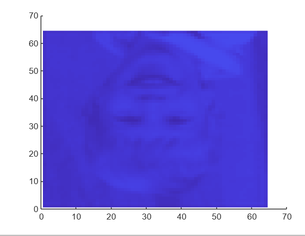
I had an error in the web version Matlab, so I exited and came back in, and this boy was plotted.
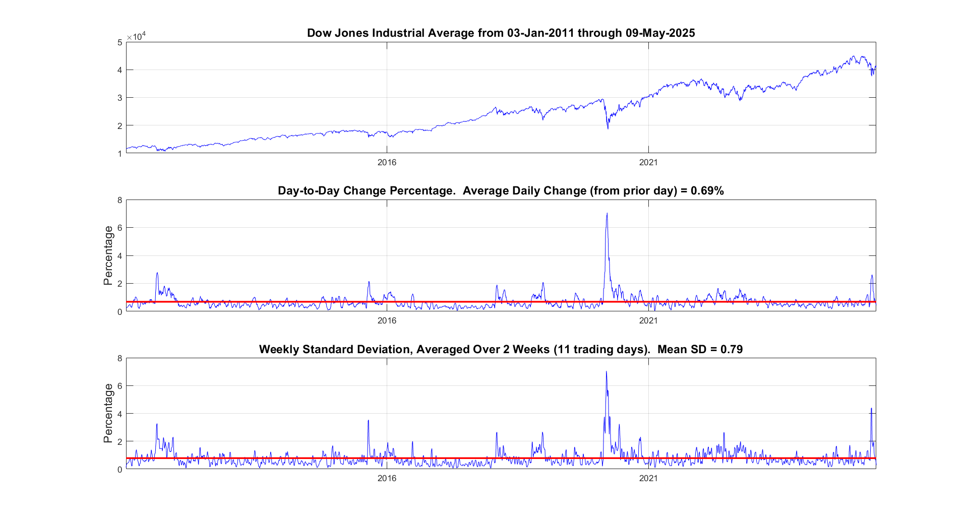
It seems like the financial news is always saying the stock market is especially volatile now. But is it really? This code will show you the daily variation from the prior day. You can see that the average daily change from one day to the next is 0.69%. So any change in the stock market from the prior day less than about 0.7% or 1% is just normal "noise"/typical variation. You can modify the code to adjust the starting date for the analysis. Data file (Excel workbook) is attached (hopefully - I attached it twice but it's not showing up yet).
% Program to plot the Dow Jones Industrial Average from 1928 to May 2025, and compute the standard deviation.
% Data available for download at https://finance.yahoo.com/quote/%5EDJI/history?p=%5EDJI
% Just set the Time Period, then find and click the download link, but you ned a paid version of Yahoo.
%
% If you have a subscription for Microsoft Office 365, you can also get historical stock prices.
% Reference: https://support.microsoft.com/en-us/office/stockhistory-function-1ac8b5b3-5f62-4d94-8ab8-7504ec7239a8#:~:text=The%20STOCKHISTORY%20function%20retrieves%20historical,Microsoft%20365%20Business%20Premium%20subscription.
% For example put this in an Excel Cell
% =STOCKHISTORY("^DJI", "1/1/2000", "5/10/2025", 0, 1, 0, 1,2,3,4, 5)
% and it will fill out a table in Excel
%====================================================================================================================
clc; % Clear the command window.
close all; % Close all figures (except those of imtool.)
imtool close all; % Close all imtool figures if you have the Image Processing Toolbox.
clear; % Erase all existing variables. Or clearvars if you want.
workspace; % Make sure the workspace panel is showing.
format long g;
format compact;
fontSize = 14;
filename = 'Dow Jones Industrial Index.xlsx';
data = readtable(filename);
% Date,Close,Open,High,Low,Volume
dates = data.Date;
closing = data.Close;
volume = data.Volume;
% Define start date and stop date
startDate = datetime(2011,1,1)
stopDate = dates(end)
selectedDates = dates > startDate;
% Extract those dates:
dates = dates(selectedDates);
closing = closing(selectedDates);
volume = volume(selectedDates);
% Plot Volume
hFigVolume = figure('Name', 'Daily Volume');
plot(dates, volume, 'b-');
grid on;
xticks(startDate:calendarDuration(5,0,0):stopDate)
title('Dow Jones Industrial Average Volume', 'FontSize', fontSize);
hFig = figure('Name', 'Daily Standard Deviation');
subplot(3, 1, 1);
plot(dates, closing, 'b-');
xticks(startDate:calendarDuration(5,0,0):stopDate)
drawnow;
grid on;
caption = sprintf('Dow Jones Industrial Average from %s through %s', dates(1), dates(end));
title(caption, 'FontSize', fontSize);
% Get the average change from one trading day to the next.
diffs = 100 * abs(closing(2:end) - closing(1:end-1)) ./ closing(1:end-1);
subplot(3, 1, 2);
averageDailyChange = mean(diffs)
% Looks pretty noisy so let's smooth it for a nicer display.
numWeeks = 4;
diffs = sgolayfilt(diffs, 2, 5*numWeeks+1);
plot(dates(2:end), diffs, 'b-');
grid on;
xticks(startDate:calendarDuration(5,0,0):stopDate)
hold on;
line(xlim, [averageDailyChange, averageDailyChange], 'Color', 'r', 'LineWidth', 2);
ylabel('Percentage', 'FontSize', fontSize);
caption = sprintf('Day-to-Day Change Percentage. Average Daily Change (from prior day) = %.2f%%', averageDailyChange);
title(caption, 'FontSize', fontSize);
drawnow;
% Get the stddev over a 5 trading day window.
sd = stdfilt(closing, ones(5, 1));
% Get it relative to the magnitude.
sd = sd ./ closing * 100;
averageVariation = mean(sd)
numWeeks = 2;
% Looks pretty noisy so let's smooth it for a nicer display.
sd = sgolayfilt(sd, 2, 5*numWeeks+1);
% Plot it.
subplot(3, 1, 3);
plot(dates, sd, 'b-');
grid on;
xticks(startDate:calendarDuration(5,0,0):stopDate)
hold on;
line(xlim, [averageVariation, averageVariation], 'Color', 'r', 'LineWidth', 2);
ylabel('Percentage', 'FontSize', fontSize);
caption = sprintf('Weekly Standard Deviation, Averaged Over %d Weeks (%d trading days). Mean SD = %.2f', ...
numWeeks, 5*numWeeks+1, averageVariation);
title(caption, 'FontSize', fontSize);
% Maximize figure window.
g = gcf;
g.WindowState = 'maximized';
I like this problem by James and have solved it in several ways. A solution by Natalie impressed me and introduced me to a new function conv2. However, it occured to me that the numerous test for the problem only cover cases of square matrices. My original solutions, and Natalie's, did niot work on rectangular matrices. I have now produced a solution which works on rectangular matrices. Thanks for this thought provoking problem James.
I wanted to turn a Markdown nested list of text labels:
- A
- B
- C
- D
- G
- H
- E
- F
- Q
into a directed graph, like this:

Here is my blog post with some related tips for doing this, including text I/O, text processing with patterns, and directed graph operations and visualization.
Large Languge model with MATLAB, a free add-on that lets you access LLMs from OpenAI, Azure, amd Ollama (to use local models) on MATLAB, has been updated to support OpenAI GPT-4.1, GPT-4.1 mini, and GPT-4.1 nano.
According to OpenAI, "These models outperform GPT‑4o and GPT‑4o mini across the board, with major gains in coding and instruction following. They also have larger context windows—supporting up to 1 million tokens of context—and are able to better use that context with improved long-context comprehension."
What would you build with the latest update?

The topic recently came up in a MATLAB Central Answers forum thread, where community members discussed how to programmatically control when the end user can close a custom app. Imagine you need to prevent app closure during a critical process but want to allow the end user to close the app afterwards. This article will guide you through the steps to add this behavior to your app.
A demo is attached containing an app with a state button that, when enabled, disables the ability to close the app.
Steps
1. Add a property that stores the state of the closure as a scalar logical value. In this example, I named the property closeEnabled. The default value in this example is true, meaning that closing is enabled. -- How to add a property to an app in app designer
properties (Access = private)
closeEnabled = true % Flag that controls ability to close app
end
2. Add a CloseRequest function to the app figure. This function is called any time there is an attempt to close the app. Within the CloseRequest function, add a condition that deletes the app when closure is enabled. -- How to add a CloseRequest function to an app figure in app designer
function UIFigureCloseRequest(app, event)
if app.closeEnabled
delete(app)
end
3. Toggle the value of the closeEnabled property as needed in your code. Imagine you have a "Process" button that initiates a process where it is crucial for the app to remain open. Set the closeEnabled flag to false (closure is disabled) at the beginning of the button's callback function and then set it to true at the end (closure is enabled).
function ProcessButtonPress(app, event)
app.closeEnabled = false;
% MY PROCESS CODE
app.closeEnabled = true;
end
Handling Errors: There is one trap to keep in mind in the example above. What if something in the callback function breaks before the app.closeEnabled is returned to true? That leaves the app in a bad state where closure is blocked. A pro move would be to use a cleanupObj to manage returning the property to true. In the example below, the task to return the closeEnabled property to true is managed by the cleanup object, which will execute that command when execution is terminated in the ProcessButtonPress function—whether execution was terminated by error or by gracefully exiting the function.
function ProcessButtonPress(app, event)
app.closeEnabled = false;
cleanupClosure = onCleanup(@()set(app,'closeEnabled',true));
% MY CODE
end
Force Closure: If the CloseRequest function is preventing an app from closing, here are a couple of ways to force a closure.
- If you have the app's handle, use delete(app) or close(app,'force'). This will also work on the app's figure handle.
- If you do not have the app's handle, you can use close('all','force') to close all figures or use findall(groot,'type','figure') to find the app's figure handle.
Provide insightful answers
9%
Provide label-AI answer
9%
Provide answer by both AI and human
21%
Do not use AI for answers
46%
Give a button "chat with copilot"
10%
use AI to draft better qustions
5%
1561 个投票
I have written, tested, and prepared a function with four subsunctions on my computer for solving one of the problems in the list of Cody problems in MathWorks in three days. Today, when I wanted to upload or copy paste the codes of the function and its subfunctions to the specified place of the problem of Cody page, I do not see a place to upload it, and the ability to copy past the codes. The total of the entire codes and their documentations is about 600 lines, which means that I cannot and it is not worth it to retype all of them in the relevent Cody environment after spending a few days. I would appreciate your guidance on how to enter the prepared codes to the desired environment in Cody.
Me: If you have parallel code and you apply this trick that only requires changing one line then it might go faster.
Reddit user: I did and it made my code 3x faster
Not bad for just one line of code!
Which makes me wonder. Could it make your MATLAB program go faster too? If you have some MATLAB code that makes use of parallel constructs like parfor or parfeval then start up your parallel pool like this
parpool("Threads")
before running your program.
The worst that will happen is you get an error message and you'll send us a bug report....or maybe it doesn't speed up much at all....
....or maybe you'll be like the Reddit user and get 3x speed-up for 10 seconds work. It must be worth a try...after all, you're using parallel computing to make your code faster right? May as well go all the way.
In an artificial benchmark I tried, I got 10x speedup! More details in my recent blog post: Parallel computing in MATLAB: Have you tried ThreadPools yet? » The MATLAB Blog - MATLAB & Simulink
Give it a try and let me know how you get on.
%% 清理环境
close all; clear; clc;
%% 模拟时间序列
t = linspace(0,12,200); % 时间从 0 到 12,分 200 个点
% 下面构造一些模拟的"峰状"数据,用于演示
% 你可以根据需要替换成自己的真实数据
rng(0); % 固定随机种子,方便复现
baseIntensity = -20; % 强度基线(z 轴的最低值)
numSamples = 5; % 样本数量
yOffsets = linspace(20,140,numSamples); % 不同样本在 y 轴上的偏移
colors = [ ...
0.8 0.2 0.2; % 红
0.2 0.8 0.2; % 绿
0.2 0.2 0.8; % 蓝
0.9 0.7 0.2; % 金黄
0.6 0.4 0.7]; % 紫
% 构造一些带多个峰的模拟数据
dataMatrix = zeros(numSamples, length(t));
for i = 1:numSamples
% 随机峰参数
peakPositions = randperm(length(t),3); % 三个峰位置
intensities = zeros(size(t));
for pk = 1:3
center = peakPositions(pk);
width = 10 + 10*rand; % 峰宽
height = 100 + 50*rand; % 峰高
% 高斯峰
intensities = intensities + height*exp(-((1:length(t))-center).^2/(2*width^2));
end
% 再加一些小随机扰动
intensities = intensities + 10*randn(size(t));
dataMatrix(i,:) = intensities;
end
%% 开始绘图
figure('Color','w','Position',[100 100 800 600],'Theme','light');
hold on; box on; grid on;
for i = 1:numSamples
% 构造 fill3 的多边形顶点
xPatch = [t, fliplr(t)];
yPatch = [yOffsets(i)*ones(size(t)), fliplr(yOffsets(i)*ones(size(t)))];
zPatch = [dataMatrix(i,:), baseIntensity*ones(size(t))];
% 使用 fill3 填充面积
hFill = fill3(xPatch, yPatch, zPatch, colors(i,:));
set(hFill,'FaceAlpha',0.8,'EdgeColor','none'); % 调整透明度、去除边框
% 在每条曲线尾部标注 Sample i
text(t(end)+0.3, yOffsets(i), dataMatrix(i,end), ...
['Sample ' num2str(i)], 'FontSize',10, ...
'HorizontalAlignment','left','VerticalAlignment','middle');
end
%% 坐标轴与视角设置
xlim([0 12]);
ylim([0 160]);
zlim([-20 350]);
xlabel('Time (sec)','FontWeight','bold');
ylabel('Frequency (Hz)','FontWeight','bold');
zlabel('Intensity','FontWeight','bold');
% 设置刻度(根据需要微调)
set(gca,'XTick',0:2:12, ...
'YTick',0:40:160, ...
'ZTick',-20:40:200);
% 设置视角(az = 水平旋转,el = 垂直旋转)
view([211 21]);
% 让三维坐标轴在后方
set(gca,'Projection','perspective');
% 如果想去掉默认的坐标轴线,也可以尝试
% set(gca,'BoxStyle','full','LineWidth',1.2);
%% 可选:在后方添加一个浅色网格平面 (示例)
% 这个与题图右上方的网格类似
[Xplane,Yplane] = meshgrid([0 12],[0 160]);
Zplane = baseIntensity*ones(size(Xplane)); % 在 Z = -20 处画一个竖直面的框
surf(Xplane, Yplane, Zplane, ...
'FaceColor',[0.95 0.95 0.9], ...
'EdgeColor','k','FaceAlpha',0.3);
%% 进一步美化(可根据需求调整)
title('3D Stacked Plot Example','FontSize',12);
constantplane("x",12,FaceColor=rand(1,3),FaceAlpha=0.5);
constantplane("y",0,FaceColor=rand(1,3),FaceAlpha=0.5);
constantplane("z",-19,FaceColor=rand(1,3),FaceAlpha=0.5);
hold off;
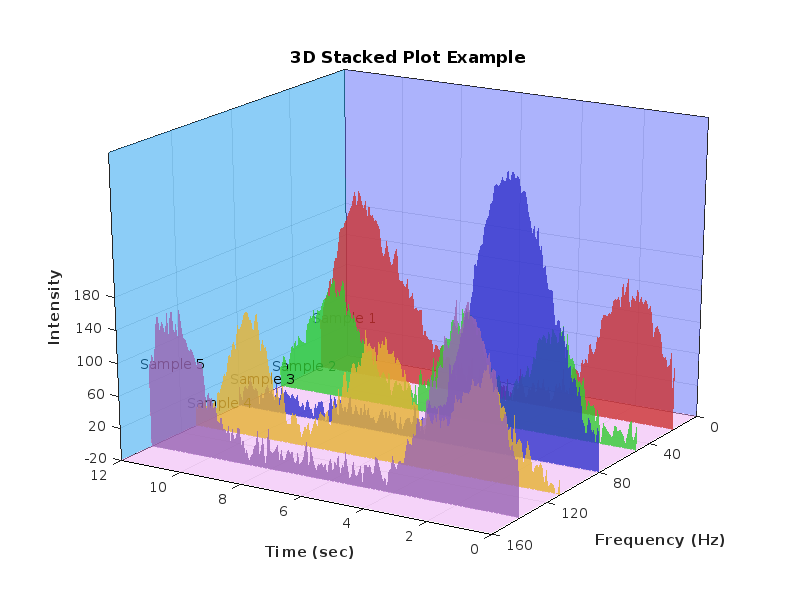
Have fun! Enjoy yourself!
Hello Community,
We're excited to announce that registration is now open for the MathWorks AUTOMOTIVE CONFERENCE 2025! This event presents a fantastic opportunity to connect with MathWorks and industry experts while exploring the latest trends in the automotive sector.
Event Details:
- Date: April 29, 2025
- Location: St. John’s Resort, Plymouth, MI
Featured Topics:
- Virtual Development
- Electrification
- Software Development
- AI in Engineering
Whether you're a professional in the automotive industry or simply interested in these cutting-edge topics, we highly encourage you to register for this conference.
We look forward to seeing you there!