搜索
I have started a blog series on the history of image display in MATLAB. If this topic interests you, and if there is something in particular you would like me to address in the series, let me know.
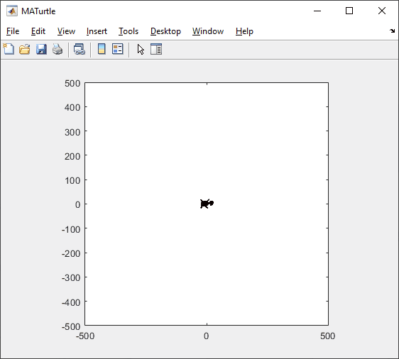
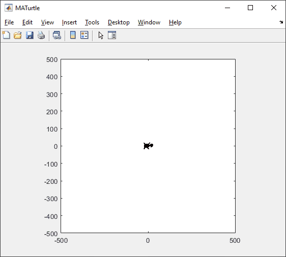
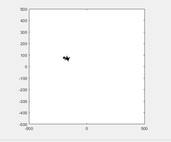
t = turtle(); % Start a turtle
t.forward(100); % Move forward by 100
t.backward(100); % Move backward by 100
t.left(90); % Turn left by 90 degrees
t.right(90); % Tur right by 90 degrees
t.goto(100, 100); % Move to (100, 100)
t.turnto(90); % Turn to 90 degrees, i.e. north
t.speed(1000); % Set turtle speed as 1000 (default: 500)
t.pen_up(); % Pen up. Turtle leaves no trace.
t.pen_down(); % Pen down. Turtle leaves a trace again.
t.color('b'); % Change line color to 'b'
t.begin_fill(FaceColor, EdgeColor, FaceAlpha); % Start filling
t.end_fill(); % End filling
t.change_icon('person.png'); % Change the icon to 'person.png'
t.clear(); % Clear the Axes
classdef turtle < handle
properties (GetAccess = public, SetAccess = private)
x = 0
y = 0
q = 0
end
properties (SetAccess = public)
speed (1, 1) double = 500
end
properties (GetAccess = private)
speed_reg = 100
n_steps = 20
ax
l
ht
im
is_pen_up = false
is_filling = false
fill_color
fill_alpha
end
methods
function obj = turtle()
figure(Name='MATurtle', NumberTitle='off')
obj.ax = axes(box="on");
hold on,
obj.ht = hgtransform();
icon = flipud(imread('turtle.png'));
obj.im = imagesc(obj.ht, icon, ...
XData=[-30, 30], YData=[-30, 30], ...
AlphaData=(255 - double(rgb2gray(icon)))/255);
obj.l = plot(obj.x, obj.y, 'k');
obj.ax.XLim = [-500, 500];
obj.ax.YLim = [-500, 500];
obj.ax.DataAspectRatio = [1, 1, 1];
obj.ax.Toolbar.Visible = 'off';
disableDefaultInteractivity(obj.ax);
end
function home(obj)
obj.x = 0;
obj.y = 0;
obj.ht.Matrix = eye(4);
end
function forward(obj, dist)
obj.step(dist);
end
function backward(obj, dist)
obj.step(-dist)
end
function step(obj, delta)
if numel(delta) == 1
delta = delta*[cosd(obj.q), sind(obj.q)];
end
if obj.is_filling
obj.fill(delta);
else
obj.move(delta);
end
end
function goto(obj, x, y)
dx = x - obj.x;
dy = y - obj.y;
obj.turnto(rad2deg(atan2(dy, dx)));
obj.step([dx, dy]);
end
function left(obj, q)
obj.turn(q);
end
function right(obj, q)
obj.turn(-q);
end
function turnto(obj, q)
obj.turn(obj.wrap_angle(q - obj.q, -180));
end
function pen_up(obj)
if obj.is_filling
warning('not available while filling')
return
end
obj.is_pen_up = true;
end
function pen_down(obj, go)
if obj.is_pen_up
if nargin == 1
obj.l(end+1) = plot(obj.x, obj.y, Color=obj.l(end).Color);
else
obj.l(end+1) = go;
end
uistack(obj.ht, 'top')
end
obj.is_pen_up = false;
end
function color(obj, line_color)
if obj.is_filling
warning('not available while filling')
return
end
obj.pen_up();
obj.pen_down(plot(obj.x, obj.y, Color=line_color));
end
function begin_fill(obj, FaceColor, EdgeColor, FaceAlpha)
arguments
obj
FaceColor = [.6, .9, .6];
EdgeColor = [0 0.4470 0.7410];
FaceAlpha = 1;
end
if obj.is_filling
warning('already filling')
return
end
obj.fill_color = FaceColor;
obj.fill_alpha = FaceAlpha;
obj.pen_up();
obj.pen_down(patch(obj.x, obj.y, [1, 1, 1], ...
EdgeColor=EdgeColor, FaceAlpha=0));
obj.is_filling = true;
end
function end_fill(obj)
if ~obj.is_filling
warning('not filling now')
return
end
obj.l(end).FaceColor = obj.fill_color;
obj.l(end).FaceAlpha = obj.fill_alpha;
obj.is_filling = false;
end
function change_icon(obj, filename)
icon = flipud(imread(filename));
obj.im.CData = icon;
obj.im.AlphaData = (255 - double(rgb2gray(icon)))/255;
end
function clear(obj)
obj.x = 0;
obj.y = 0;
delete(obj.ax.Children(2:end));
obj.l = plot(0, 0, 'k');
obj.ht.Matrix = eye(4);
end
end
methods (Access = private)
function animated_step(obj, delta, q, initFcn, updateFcn)
arguments
obj
delta
q
initFcn = @() []
updateFcn = @(~, ~) []
end
dx = delta(1)/obj.n_steps;
dy = delta(2)/obj.n_steps;
dq = q/obj.n_steps;
pause_duration = norm(delta)/obj.speed/obj.speed_reg;
initFcn();
for i = 1:obj.n_steps
updateFcn(dx, dy);
obj.ht.Matrix = makehgtform(...
translate=[obj.x + dx*i, obj.y + dy*i, 0], ...
zrotate=deg2rad(obj.q + dq*i));
pause(pause_duration)
drawnow limitrate
end
obj.x = obj.x + delta(1);
obj.y = obj.y + delta(2);
end
function obj = turn(obj, q)
obj.animated_step([0, 0], q);
obj.q = obj.wrap_angle(obj.q + q, 0);
end
function move(obj, delta)
initFcn = @() [];
updateFcn = @(dx, dy) [];
if ~obj.is_pen_up
initFcn = @() initializeLine();
updateFcn = @(dx, dy) obj.update_end_point(obj.l(end), dx, dy);
end
function initializeLine()
obj.l(end).XData(end+1) = obj.l(end).XData(end);
obj.l(end).YData(end+1) = obj.l(end).YData(end);
end
obj.animated_step(delta, 0, initFcn, updateFcn);
end
function obj = fill(obj, delta)
initFcn = @() initializePatch();
updateFcn = @(dx, dy) obj.update_end_point(obj.l(end), dx, dy);
function initializePatch()
obj.l(end).Vertices(end+1, :) = obj.l(end).Vertices(end, :);
obj.l(end).Faces = 1:size(obj.l(end).Vertices, 1);
end
obj.animated_step(delta, 0, initFcn, updateFcn);
end
end
methods (Static, Access = private)
function update_end_point(l, dx, dy)
l.XData(end) = l.XData(end) + dx;
l.YData(end) = l.YData(end) + dy;
end
function q = wrap_angle(q, min_angle)
q = mod(q - min_angle, 360) + min_angle;
end
end
end
I would like to zoom directly on the selected region when using  on my image created with image or imagesc. First of all, I would recommend using image or imagesc and not imshow for this case, see comparison here: Differences between imshow() and image()? However when zooming Stretch-to-Fill behavior happens and I don't want that. Try range zoom to image generated by this code:
fig = uifigure;
ax = uiaxes(fig);
im = imread("peppers.png");
h = imagesc(im,"Parent",ax);
axis(ax,'tight', 'off')
I can fix that with manualy setting data aspect ratio:
daspect(ax,[1 1 1])
However, I need this code to run automatically after zooming. So I create zoom object and ActionPostCallback which is called everytime after I zoom, see zoom - ActionPostCallback.
z = zoom(ax);
z.ActionPostCallback = @(fig,ax) daspect(ax.Axes,[1 1 1]);
If you need, you can also create ActionPreCallback which is called everytime before I zoom, see zoom - ActionPreCallback.
z.ActionPreCallback = @(fig,ax) daspect(ax.Axes,'auto');
Code written and run in R2025a.
This week's Graphics and App Building blog article guides chart authors and app builders through the process of designing for a specific theme or creating theme-responsive charts and apps.
- Learn how dark theme may impacts charts and apps
- Discover best practices for theme-adaptive workflows
- Step-by-step examples for both script-based plots and advanced custom charts and UI components
- Discover new tools like ThemeChangedFcn, getTheme, and fliplightness
I'm planning to start a personal scientific software project. I used to be familiar with Matlab (quite some time ago), so Matlab would be my first choice. But I keep hearing that Matlab is old stuff and I should use Julia or something like that. I wouldn't find learning Julia difficult, so familiarity with Matlab is not an important factor. Neither is cost, because I can afford a home license for Matlab, Simulink and a few toolboxes. So I'm thinking. Please give me your input! Why should I use Matlab in 2025 instead of alternatives?
I’m quite curious as to why this particular email was sent directly to my personal inbox. I have never actively subscribed to any online or offline training services nor clicked on any related marketing links. Could it be that because I frequently visit the official MATLAB forums, someone has identified me as a potential customer for their targeted promotions?
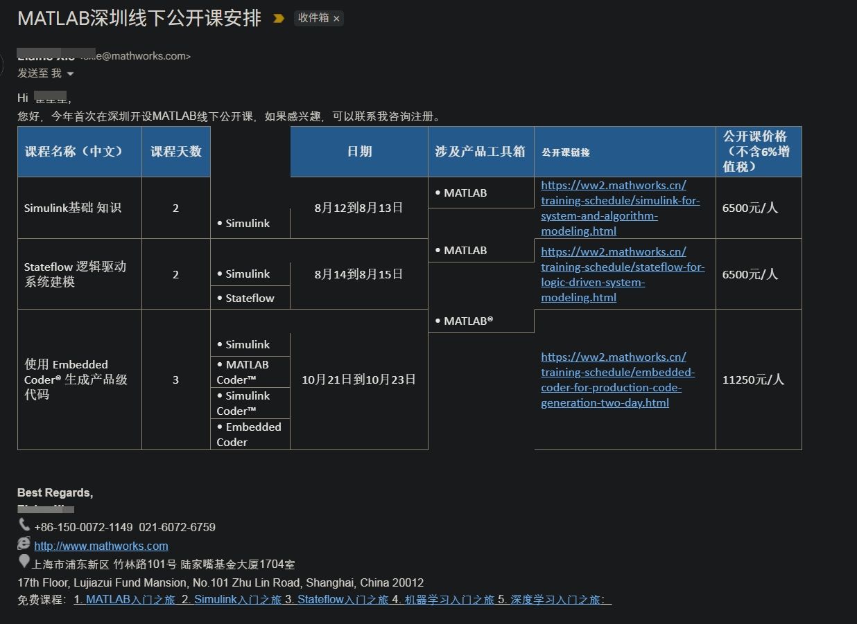
I’d love to hear your thoughts and start a discussion on this!
I am thrilled python interoperability now seems to work for me with my APPLE M1 MacBookPro and MATLAB V2025a. The available instructions are still, shall we say, cryptic. Here is a summary of my interaction with GPT 4o to get this to work.
===========================================================
MATLAB R2025a + Python (Astropy) Integration on Apple Silicon (M1/M2/M3 Macs)
===========================================================
Author: D. Carlsmith, documented with ChatGPT
Last updated: July 2025
This guide provides full instructions, gotchas, and workarounds to run Python 3.10 with MATLAB R2025a (Apple Silicon/macOS) using native ARM64 Python and calling modules like Astropy, Numpy, etc. from within MATLAB.
===========================================================
Overview
===========================================================
- MATLAB R2025a on Apple Silicon (M1/M2/M3) runs as "maca64" (native ARM64).
- To call Python from MATLAB, the Python interpreter must match that architecture (ARM64).
- Using Intel Python (x86_64) with native MATLAB WILL NOT WORK.
- The cleanest solution: use Miniforge3 (Conda-forge's lightweight ARM64 distribution).
===========================================================
1. Install Miniforge3 (ARM64-native Conda)
===========================================================
In Terminal, run:
curl -LO https://github.com/conda-forge/miniforge/releases/latest/download/Miniforge3-MacOSX-arm64.sh
bash Miniforge3-MacOSX-arm64.sh
Follow prompts:
- Press ENTER to scroll through license.
- Type "yes" when asked to accept the license.
- Press ENTER to accept the default install location: ~/miniforge3
- When asked:
Do you wish to update your shell profile to automatically initialize conda? [yes|no]
Type: yes
===========================================================
2. Restart Terminal and Create a Python Environment for MATLAB
===========================================================
Run the following:
conda create -n matlab python=3.10 astropy numpy -y
conda activate matlab
Verify the Python path:
which python
Expected output:
/Users/YOURNAME/miniforge3/envs/matlab/bin/python
===========================================================
3. Verify Python + Astropy From Terminal
===========================================================
Run:
python -c "import astropy; print(astropy.__version__)"
Expected output:
6.x.x (or similar)
===========================================================
4. Configure MATLAB to Use This Python
===========================================================
In MATLAB R2025a (Apple Silicon):
clear classes
pyenv('Version', '/Users/YOURNAME/miniforge3/envs/matlab/bin/python')
py.sys.version
You should see the Python version printed (e.g. 3.10.18). No error means it's working.
===========================================================
5. Gotchas and Their Solutions
===========================================================
❌ Error: Python API functions are not available
→ Cause: Wrong architecture or broken .dylib
→ Fix: Use Miniforge ARM64 Python. DO NOT use Intel Anaconda.
❌ Error: Invalid text character (↑ points at __version__)
→ Cause: MATLAB can’t parse double underscores typed or pasted
→ Fix: Use: py.getattr(module, '__version__')
❌ Error: Unrecognized method 'separation' or 'sec'
→ Cause: MATLAB can't reflect dynamic Python methods
→ Fix: Use: py.getattr(obj, 'method')(args)
===========================================================
6. Run Full Verification in MATLAB
===========================================================
Paste this into MATLAB:
% Set environment
clear classes
pyenv('Version', '/Users/YOURNAME/miniforge3/envs/matlab/bin/python');
% Import modules
coords = py.importlib.import_module('astropy.coordinates');
time_mod = py.importlib.import_module('astropy.time');
table_mod = py.importlib.import_module('astropy.table');
% Astropy version
ver = char(py.getattr(py.importlib.import_module('astropy'), '__version__'));
disp(['Astropy version: ', ver]);
% SkyCoord angular separation
c1 = coords.SkyCoord('10h21m00s', '+41d12m00s', pyargs('frame', 'icrs'));
c2 = coords.SkyCoord('10h22m00s', '+41d15m00s', pyargs('frame', 'icrs'));
sep_fn = py.getattr(c1, 'separation');
sep = sep_fn(c2);
arcsec = double(sep.to('arcsec').value);
fprintf('Angular separation = %.3f arcsec\n', arcsec);
% Time difference in seconds
Time = time_mod.Time;
t1 = Time('2025-01-01T00:00:00', pyargs('format','isot','scale','utc'));
t2 = Time('2025-01-02T00:00:00', pyargs('format','isot','scale','utc'));
dt = py.getattr(t2, '__sub__')(t1);
seconds = double(py.getattr(dt, 'sec'));
fprintf('Time difference = %.0f seconds\n', seconds);
% Astropy table display
tbl = table_mod.Table(pyargs('names', {'a','b'}, 'dtype', {'int','float'}));
tbl.add_row({1, 2.5});
tbl.add_row({2, 3.7});
disp(tbl);
===========================================================
7. Optional: Automatically Configure Python in startup.m
===========================================================
To avoid calling pyenv() every time, edit your MATLAB startup:
edit startup.m
Add:
try
pyenv('Version', '/Users/YOURNAME/miniforge3/envs/matlab/bin/python');
catch
warning("Python already loaded.");
end
===========================================================
8. Final Notes
===========================================================
- This setup avoids all architecture mismatches.
- It uses a clean, minimal ARM64 Python that integrates seamlessly with MATLAB.
- Do not mix Anaconda (Intel) with Apple Silicon MATLAB.
- Use py.getattr for any Python attribute containing underscores or that MATLAB can't resolve.
You can now run NumPy, Astropy, Pandas, Astroquery, Matplotlib, and more directly from MATLAB.
===========================================================
One of MATLAB's strengths is how easy it is to document a custom function/class. The first continuous comment block is automatially displayed by the help and doc functions, with some neat automatic formatting. For example:
% myFunc My example function
%
% This function does not do anything yet, but one day will be great. For
% example, you will be able to type:
% out=myFunc(in1,in2);
% and something cool will happen.
%
% See also otherFunc
function varargout=myFunc(varargin)
% actual code
end
will have a link to the documentation for "otherFunc", assuming that file exists. Class documentation is nicely broken up into a header (with "See also" support) followed by a property and method summary.
All the above works great with one big exception: apart from highlighting uses of the file's name, there is no way to display anything but pure text. No Markdown, no LateX, and so forth. It is possible to sneak an HTML link into the comment block, calling a MATLAB command that can display a live script with fancy formatting. I have done this in the past, although it can be a little tricky for files inside a package/namespace (folders beginning with '+').
I can envision a system where fancy documentation would be buried inside an "example" subfolder where "myFunc.m" is located. Invoking "showExample myFunc", where "showExample" is a to-be-written utility, would look for a live script inside the appropriate subfolder, make a local copy for the user to tinker with, and then display that local copy in the MATLAB editor. Since the actual function function and its example woulld obviously inside a Git repository, text-based live scripts would be used instead of an *.mlx file.
Again, this all works fine on its fine on its own, but it would be very difficult to replicate the "See also" capability or the other features of the standard doc function. So what are we to do? Is there a clever way to add another block to a standard comment block "See examples" that would automatically detect scripts in a subfolder of function/class being queried?
I know there is a way to incorporate custom documentation into MATLAB help system. This is much too cumbersome for my purposes, where many functions/classes are being added/edited all the time. The existing doc system covers maybe 80% of my needs, but sometimes a little math (LaTeX) would go a long way on explaining how things work.
Are you a dark mode enthusiast or are you curious about how it’s shaping MATLAB graphics? Check out the latest article in the MATLAB Graphics and App Building blog.
🔹 User Insights: find out how user surveys influenced the development of graphics themes
🔹 Learn three ways to switch between light and dark themes for figures
🔹 Understand how custom and default colors behave across themes
🔹 Download a handy cheat sheet for working with themes in your graphics and apps.
Hey MATLAB enthusiasts!
I just stumbled upon this hilariously effective GitHub repo for image deformation using Moving Least Squares (MLS)—and it’s pure gold for anyone who loves playing with pixels! 🎨✨
- Real-Time Magic ✨
- Precomputes weights and deformation data upfront, making it blazing fast for interactive edits. Drag control points and watch the image warp like rubber! (2)
- Supports affine, similarity, and rigid deformations—because why settle for one flavor of chaos?
- Single-File Simplicity 🧩
- All packed into one clean MATLAB class (mlsImageWarp.m).
- Endless Fun Use Cases 🤹
- Turn your pet’s photo into a Picasso painting.
- "Fix" your friend’s smile... aggressively.
- Animate static images with silly deformations (1).
Try the Demo!
automatisation du calcul du SSDE(Size Specific Dose Estimate )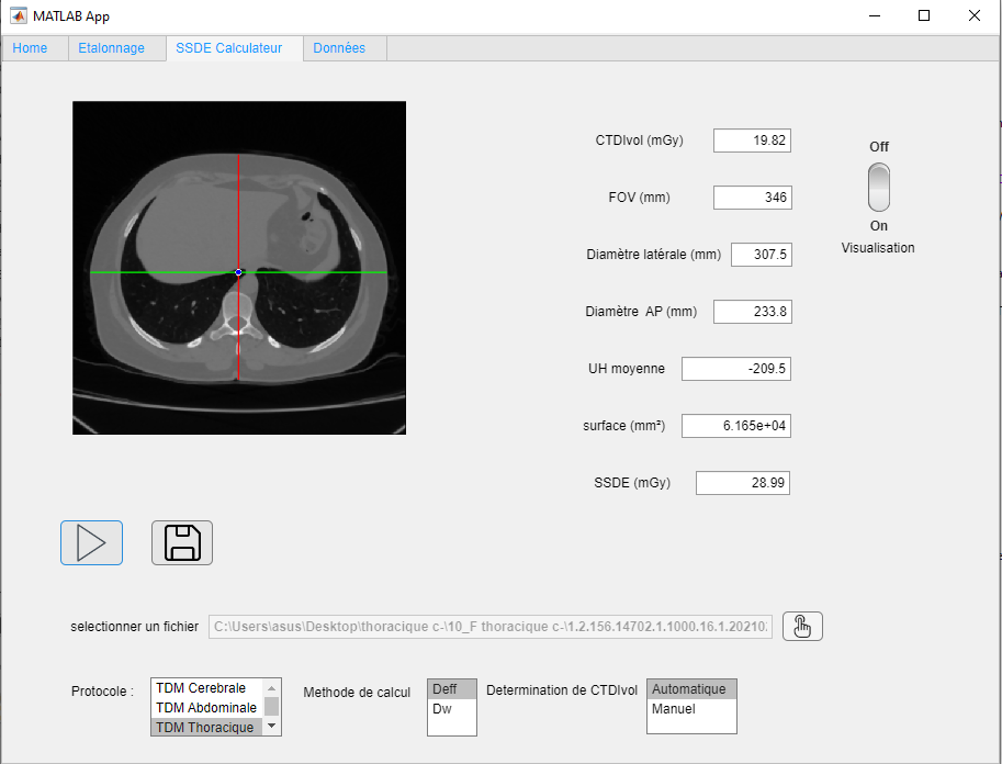
The new figure toolstrip in R2025a was designed from multiple feedback cycles with MATLAB users. See the latest article in the Graphics and App Building blog to see the evolution of the figure toolbar from 1996-2025, learn how user feedback shaped the new toolstrip, and check out the new code-generation feature that makes interactive data exporation reproducible.
I rarely use MATLAB.
10%
use MATLAB almost every day.
55%
use MATLAB once every 2-3 days.
10%
only use when specific task require
25%
20 个投票
For the last day or two, I've been getting "upstream" and other various errors on Answers. Seems to come and go. Anyone else having similar issues?
You are not a jedi yet !
20%
We not grant u the rank of master !
0%
Ready are u? What knows u of ready?
0%
May the Force be with you !
80%
5 个投票
In a discussion on LInkedin about my recent blog post, Do these 3 things to increase the reach of your open source MATLAB toolbox, I was asked by "Could you elaborate on why someone might consider opening/sharing their code? Thinking of early-career researchers, what might be in it for them?"
I'll give my answer here but I'm more interested in yours. How would you have answered this?
This is what I said:
- It's the right thing to do scientifically. A computational paper is essentially just an advertisement of what you've done. The code contains vital details about how you actually did it. A computational paper is incomplete without the code.
- If you only describe your algorithm in a paper, I have to implement it before I can apply your research to my problem. If you share the code, I can get started much more quickly using your research. This means I publish faster and since I am a good scientist, this means you get cited faster.
- Other scientists start off as users of your code. This leads to citations. Over time, some of them start deeply using and modifying your code, this leads to collaborators.
- Once you decide to share code via something like GitHub, you quickly start adopting good software engineering practices without initially realizing it. This improves the quality of your research since adopting good software practices makes it more likely that your software will give the right answers.
That last point can be a little hard to get your head around sometimes. Even if all you do is use file upload to get your stuff onto GitHub (i.e. you're not using git properly yet) you will start to naturally converge towards better code.
Why? Because as soon as you share code, you have to solve the problem of getting it to run on someone else's machine.
A trivial example concerns hard coded paths, for example. If you only ever run it on your machine then having a line like datafile = "C:\Mystuff\data.csv" always works but it breaks as soon as I try to run it on my machine. You'll look at this and think "Maybe there's a better way to do that".
Similarly dependencies. Your Path may be full of stuff that isn't present on my machine. As soon as I try to run your code, it won't work and you'll have to figure out how to handle dependencies in a reproducible way.
Documentation! An empty README.md is no good if you expect me to know how to use your code. You at least have to say something like "To run this, type runme(N) into MATLAB where N is the size of the model...etc etc)
The act of sharing, and dealing with the consequences, leads to much better code than if you keep it to yourself.
The MATLAB R2025a release gave figures a makeover. @Brian Knolhoff, a developer on the Figure Infrastructure and Services team, reviews the new Figure Container in the Graphics and App Building blog.
Learn the four ways to tile figures, what docking means, and other new features.
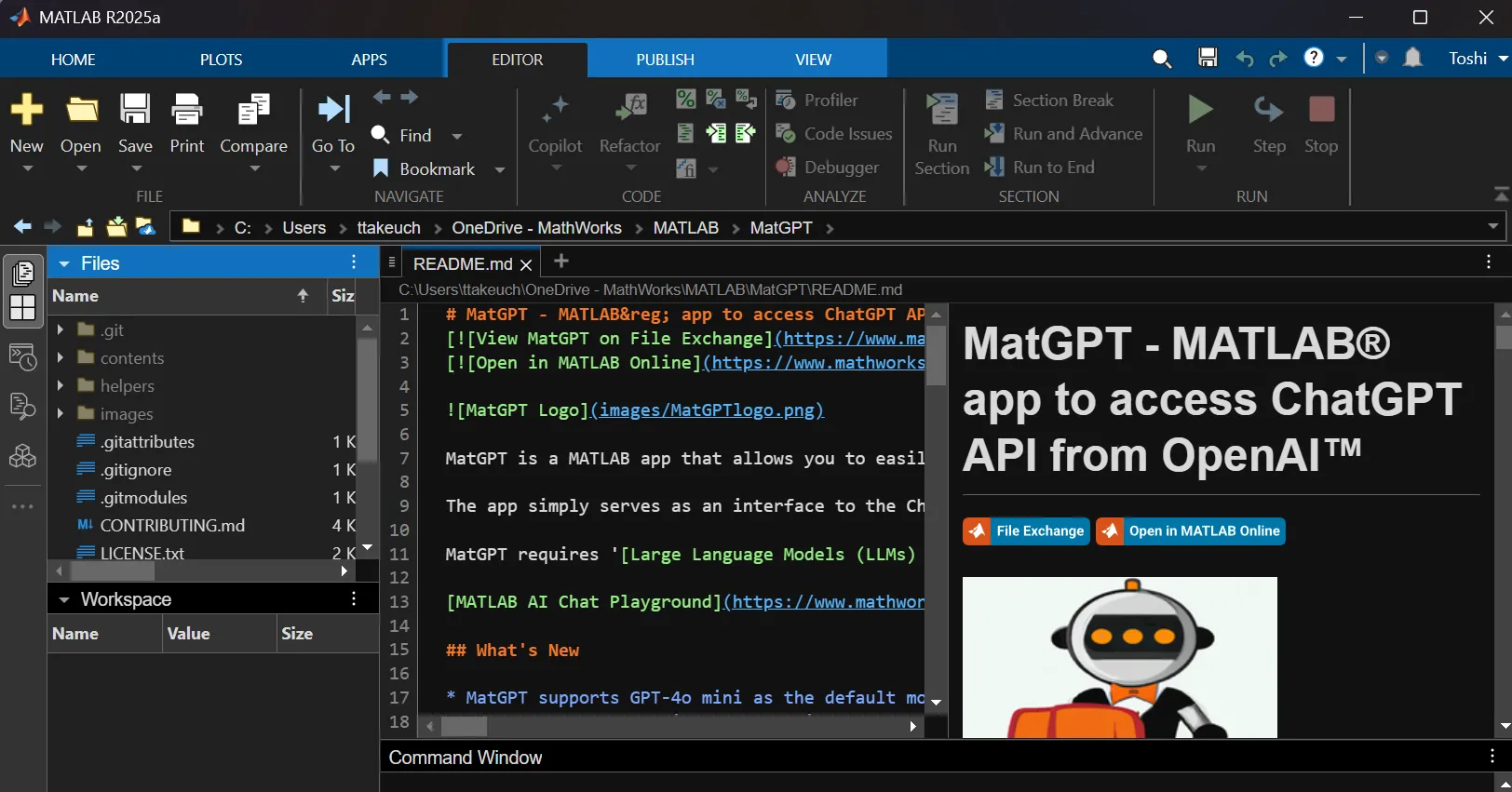
In case you missed it in my overview of the MATLAB R2025a release, Markdown support has been greatly improved. This picture says it all
I saw this on Reddit and thought of the past mini-hack contests. We have a few folks here who can do something similar with MATLAB.
The Graphics and App Building Blog just launched its first article on R2025a features, authored by Chris Portal, the director of engineering for the MATLAB graphics and app building teams.
Over the next few months, we'll publish a series of articles that showcase our updated graphics system, introduce new tools and features, and provide valuable references enriched by the perspectives of those involved in their development.
To stay updated, you can subscribe to the blog (look for the option in the upper left corner of the blog page). We also encourage you to join the conversation—your comments and questions under each article help shape the discussion and guide future content.