主要内容
Results for
We are modeling the introduction of a novel pathogen into a completely susceptible population. In the cells below, I have provided you with the Matlab code for a simple stochastic SIR model, implemented using the "GillespieSSA" function
Simulating the stochastic model 100 times for 
Since γ is 0.4 per day,  per day
% Define the parameters
beta = 0.36;
gamma = 0.4;
n_sims = 100;
tf = 100; % Time frame changed to 100
% Calculate R0
R0 = beta / gamma
% Initial state values
initial_state_values = [1000000; 1; 0; 0]; % S, I, R, cum_inc
% Define the propensities and state change matrix
a = @(state) [beta * state(1) * state(2) / 1000000, gamma * state(2)];
nu = [-1, 0; 1, -1; 0, 1; 0, 0];
% Define the Gillespie algorithm function
function [t_values, state_values] = gillespie_ssa(initial_state, a, nu, tf)
t = 0;
state = initial_state(:); % Ensure state is a column vector
t_values = t;
state_values = state';
while t < tf
rates = a(state);
rate_sum = sum(rates);
if rate_sum == 0
break;
end
tau = -log(rand) / rate_sum;
t = t + tau;
r = rand * rate_sum;
cum_sum_rates = cumsum(rates);
reaction_index = find(cum_sum_rates >= r, 1);
state = state + nu(:, reaction_index);
% Update cumulative incidence if infection occurred
if reaction_index == 1
state(4) = state(4) + 1; % Increment cumulative incidence
end
t_values = [t_values; t];
state_values = [state_values; state'];
end
end
% Function to simulate the stochastic model multiple times and plot results
function simulate_stoch_model(beta, gamma, n_sims, tf, initial_state_values, R0, plot_type)
% Define the propensities and state change matrix
a = @(state) [beta * state(1) * state(2) / 1000000, gamma * state(2)];
nu = [-1, 0; 1, -1; 0, 1; 0, 0];
% Set random seed for reproducibility
rng(11);
% Initialize plot
figure;
hold on;
for i = 1:n_sims
[t, output] = gillespie_ssa(initial_state_values, a, nu, tf);
% Check if the simulation had only one step and re-run if necessary
while length(t) == 1
[t, output] = gillespie_ssa(initial_state_values, a, nu, tf);
end
if strcmp(plot_type, 'cumulative_incidence')
plot(t, output(:, 4), 'LineWidth', 2, 'Color', rand(1, 3));
elseif strcmp(plot_type, 'prevalence')
plot(t, output(:, 2), 'LineWidth', 2, 'Color', rand(1, 3));
end
end
xlabel('Time (days)');
if strcmp(plot_type, 'cumulative_incidence')
ylabel('Cumulative Incidence');
ylim([0 inf]);
elseif strcmp(plot_type, 'prevalence')
ylabel('Prevalence of Infection');
ylim([0 50]);
end
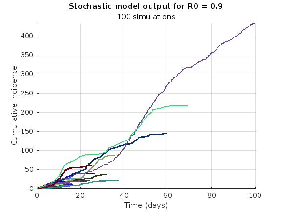
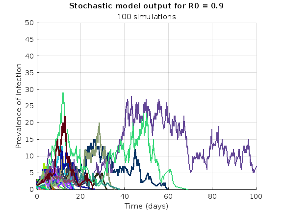
title(['Stochastic model output for R0 = ', num2str(R0)]);
subtitle([num2str(n_sims), ' simulations']);
xlim([0 tf]);
grid on;
hold off;
end
% Simulate the model 100 times and plot cumulative incidence
simulate_stoch_model(beta, gamma, n_sims, tf, initial_state_values, R0, 'cumulative_incidence');
% Simulate the model 100 times and plot prevalence
simulate_stoch_model(beta, gamma, n_sims, tf, initial_state_values, R0, 'prevalence');
Twitch built an entire business around letting you watch over someone's shoulder while they play video games. I feel like we should be able to make at least a few videos where we get to watch over someone's shoulder while they solve Cody problems. I would pay good money for a front-row seat to watch some of my favorite solvers at work. Like, I want to know, did Alfonso Nieto-Castonon just sit down and bang out some of those answers, or did he have to think about it for a while? What was he thinking about while he solved it? What resources was he drawing on? There's nothing like watching a master craftsman at work.
I can imagine a whole category of Cody videos called "How I Solved It". I tried making one of these myself a while back, but as far as I could tell, nobody else made one.
Here's the direct link to the video: https://www.youtube.com/watch?v=hoSmO1XklAQ
I hereby challenge you to make a "How I Solved It" video and post it here. If you make one, I'll make another one.
Base case:
Suppose you need to do a computation many times. We are going to assume that this computation cannot be vectorized. The simplest case is to use a for loop:
number_of_elements = 1e6;
test_fcn = @(x) sqrt(x) / x;
tic
for i = 1:number_of_elements
x(i) = test_fcn(i);
end
t_forward = toc;
disp(t_forward + " seconds")
Preallocation:
This can easily be sped up by preallocating the variable that houses results:
tic
x = zeros(number_of_elements, 1);
for i = 1:number_of_elements
x(i) = test_fcn(i);
end
t_forward_prealloc = toc;
disp(t_forward_prealloc + " seconds")
In this example, preallocation speeds up the loop by a factor of about three to four (running in R2024a). Comment below if you get dramatically different results.
disp(sprintf("%.1f", t_forward / t_forward_prealloc))
Run it in reverse:
Is there a way to skip the explicit preallocation and still be fast? Indeed, there is.
clear x
tic
for i = number_of_elements:-1:1
x(i) = test_fcn(i);
end
t_backward = toc;
disp(t_backward + " seconds")
By running the loop backwards, the preallocation is implicitly performed during the first iteration and the loop runs in about the same time (within statistical noise):
disp(sprintf("%.2f", t_forward_prealloc / t_backward))
Do you get similar results when running this code? Let us know your thoughts in the comments below.
Beneficial side effect:
Have you ever had to use a for loop to delete elements from a vector? If so, keeping track of index offsets can be tricky, as deleting any element shifts all those that come after. By running the for loop in reverse, you don't need to worry about index offsets while deleting elements.
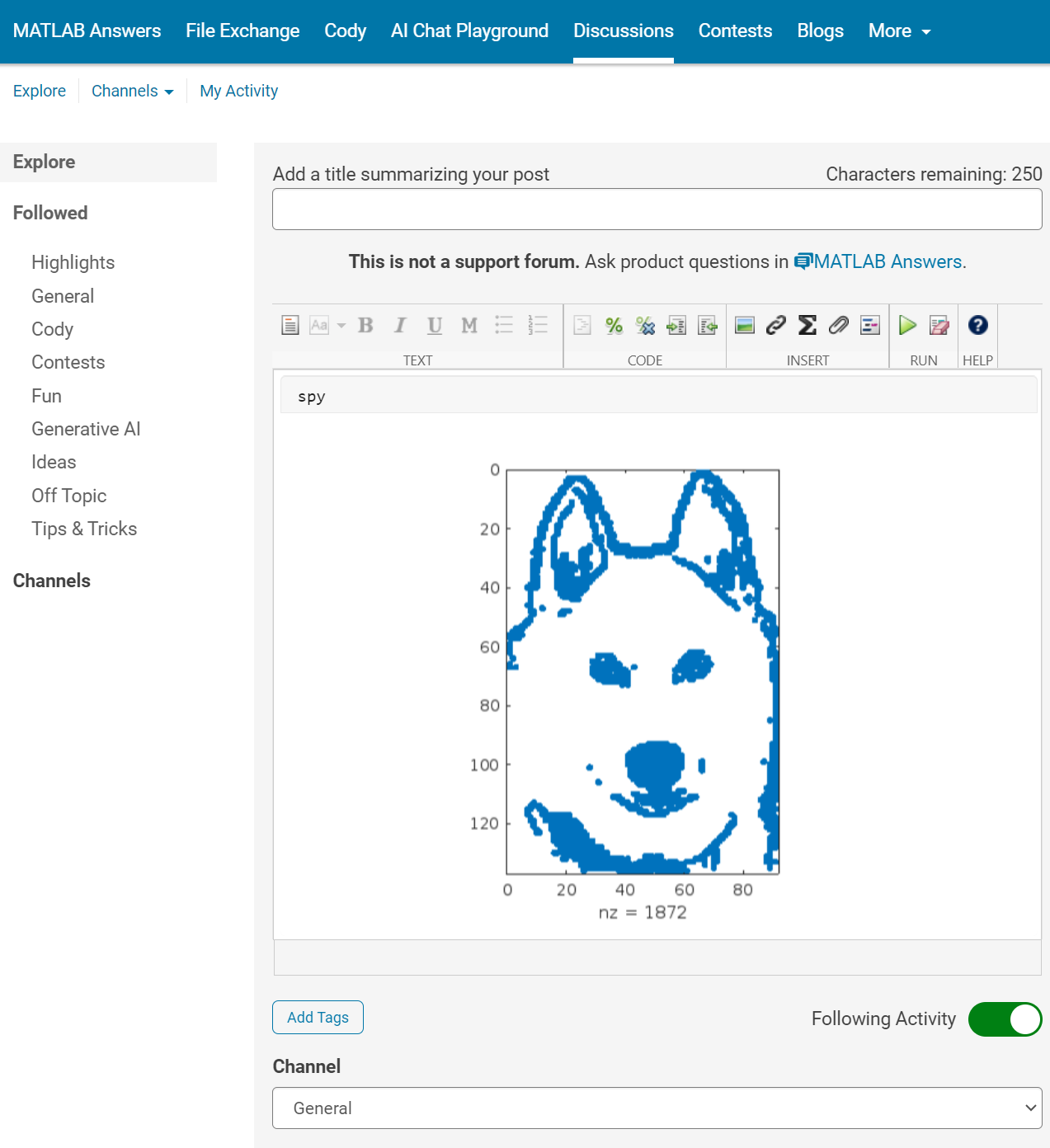
We're thrilled to share an exciting update with our community: the 'Run Code' feature is now available in the Discussions area!
Simply insert your code into the editor and press the green triangle button to run it. Your code will execute using the latest MATLAB R24a version, and it supports most common toolboxes. Moreover, this innovative feature allows for the running of attached files, further enhancing its utility and flexibility.
The ‘run code’ feature was first introduced in MATLAB Answers. Encouraged by the positive feedback and at the request of our community members, we are now expanding the availability of this feature to more areas within our community.
As always, your feedback is crucial to us, so please don't hesitate to share your thoughts and experiences by leaving a comment.
The Ans Hack is a dubious way to shave a few points off your solution score. Instead of a standard answer like this
function y = times_two(x)
y = 2*x;
end
you would do this
function ans = times_two(x)
2*x;
end
The ans variable is automatically created when there is no left-hand side to an evaluated expression. But it makes for an ugly function. I don't think anyone actually defends it as a good practice. The question I would ask is: is it so offensive that it should be specifically disallowed by the rules? Or is it just one of many little hacks that you see in Cody, inelegant but tolerable in the context of the surrounding game?
Incidentally, I wrote about the Ans Hack long ago on the Community Blog. Dealing with user-unfriendly code is also one of the reasons we created the Head-to-Head voting feature. Some techniques are good for your score, and some are good for your code readability. You get to decide with you care about.
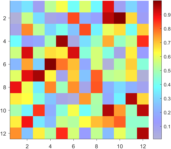
Many times when ploting, we not only need to set the color of the plot, but also its
transparency, Then how we set the alphaData of colorbar at the same time ?
It seems easy to do so :
data = rand(12,12);
% Transparency range 0-1, .3-1 for better appearance here
AData = rescale(- data, .3, 1);
% Draw an imagesc with numerical control over colormap and transparency
imagesc(data, 'AlphaData',AData);
colormap(jet);
ax = gca;
ax.DataAspectRatio = [1,1,1];
ax.TickDir = 'out';
ax.Box = 'off';
% get colorbar object
CBarHdl = colorbar;
pause(1e-16)
% Modify the transparency of the colorbar
CData = CBarHdl.Face.Texture.CData;
ALim = [min(min(AData)), max(max(AData))];
CData(4,:) = uint8(255.*rescale(1:size(CData, 2), ALim(1), ALim(2)));
CBarHdl.Face.Texture.ColorType = 'TrueColorAlpha';
CBarHdl.Face.Texture.CData = CData;
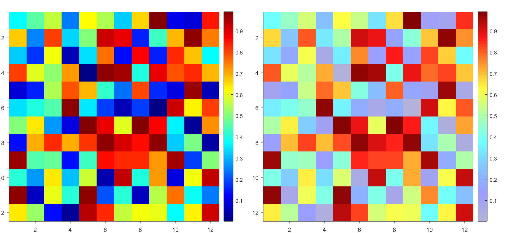
But !!!!!!!!!!!!!!! We cannot preserve the changes when saving them as images :
It seems that when saving plots, the `Texture` will be refresh, but the `Face` will not :
however, object Face only have 4 colors to change(The four corners of a quadrilateral), how
can we set more colors ??
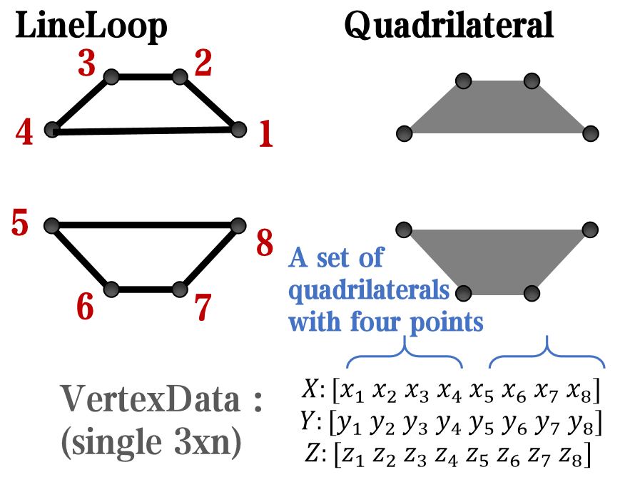
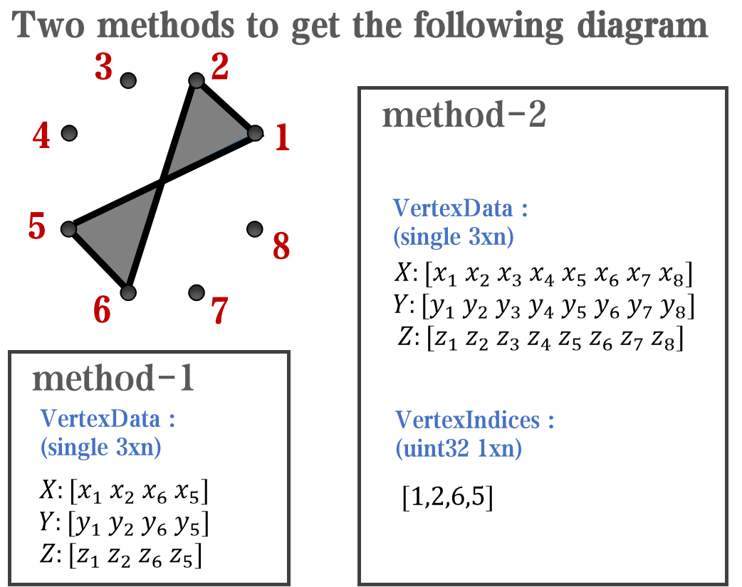
`Face` is a quadrilateral object, and we can change the `VertexData` to draw more than one little quadrilaterals:
data = rand(12,12);
% Transparency range 0-1, .3-1 for better appearance here
AData = rescale(- data, .3, 1);
%Draw an imagesc with numerical control over colormap and transparency
imagesc(data, 'AlphaData',AData);
colormap(jet);
ax = gca;
ax.DataAspectRatio = [1,1,1];
ax.TickDir = 'out';
ax.Box = 'off';
% get colorbar object
CBarHdl = colorbar;
pause(1e-16)
% Modify the transparency of the colorbar
CData = CBarHdl.Face.Texture.CData;
ALim = [min(min(AData)), max(max(AData))];
CData(4,:) = uint8(255.*rescale(1:size(CData, 2), ALim(1), ALim(2)));
warning off
CBarHdl.Face.ColorType = 'TrueColorAlpha';
VertexData = CBarHdl.Face.VertexData;
tY = repmat((1:size(CData,2))./size(CData,2), [4,1]);
tY1 = tY(:).'; tY2 = tY - tY(1,1); tY2(3:4,:) = 0; tY2 = tY2(:).';
tM1 = [tY1.*0 + 1; tY1; tY1.*0 + 1];
tM2 = [tY1.*0; tY2; tY1.*0];
CBarHdl.Face.VertexData = repmat(VertexData, [1,size(CData,2)]).*tM1 + tM2;
CBarHdl.Face.ColorData = reshape(repmat(CData, [4,1]), 4, []);
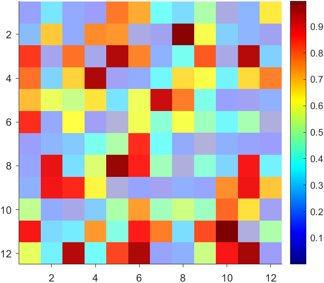
The higher the value, the more transparent it becomes
data = rand(12,12);
AData = rescale(- data, .3, 1);
imagesc(data, 'AlphaData',AData);
colormap(jet);
ax = gca;
ax.DataAspectRatio = [1,1,1];
ax.TickDir = 'out';
ax.Box = 'off';
CBarHdl = colorbar;
pause(1e-16)
CData = CBarHdl.Face.Texture.CData;
ALim = [min(min(AData)), max(max(AData))];
CData(4,:) = uint8(255.*rescale(size(CData, 2):-1:1, ALim(1), ALim(2)));
warning off
CBarHdl.Face.ColorType = 'TrueColorAlpha';
VertexData = CBarHdl.Face.VertexData;
tY = repmat((1:size(CData,2))./size(CData,2), [4,1]);
tY1 = tY(:).'; tY2 = tY - tY(1,1); tY2(3:4,:) = 0; tY2 = tY2(:).';
tM1 = [tY1.*0 + 1; tY1; tY1.*0 + 1];
tM2 = [tY1.*0; tY2; tY1.*0];
CBarHdl.Face.VertexData = repmat(VertexData, [1,size(CData,2)]).*tM1 + tM2;
CBarHdl.Face.ColorData = reshape(repmat(CData, [4,1]), 4, []);
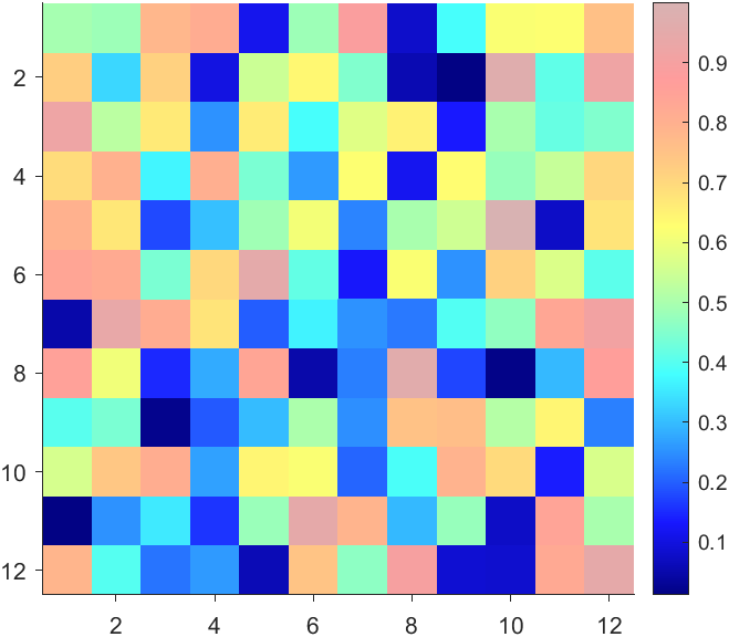
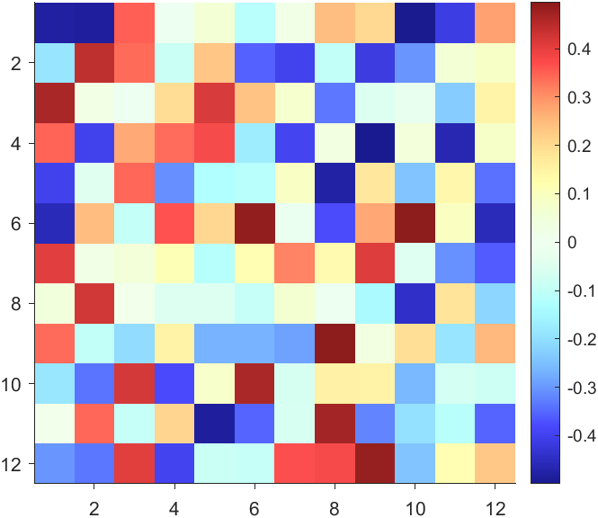
More transparent in the middle
data = rand(12,12) - .5;
AData = rescale(abs(data), .1, .9);
imagesc(data, 'AlphaData',AData);
colormap(jet);
ax = gca;
ax.DataAspectRatio = [1,1,1];
ax.TickDir = 'out';
ax.Box = 'off';
CBarHdl = colorbar;
pause(1e-16)
CData = CBarHdl.Face.Texture.CData;
ALim = [min(min(AData)), max(max(AData))];
CData(4,:) = uint8(255.*rescale(abs((1:size(CData, 2)) - (1 + size(CData, 2))/2), ALim(1), ALim(2)));
warning off
CBarHdl.Face.ColorType = 'TrueColorAlpha';
VertexData = CBarHdl.Face.VertexData;
tY = repmat((1:size(CData,2))./size(CData,2), [4,1]);
tY1 = tY(:).'; tY2 = tY - tY(1,1); tY2(3:4,:) = 0; tY2 = tY2(:).';
tM1 = [tY1.*0 + 1; tY1; tY1.*0 + 1];
tM2 = [tY1.*0; tY2; tY1.*0];
CBarHdl.Face.VertexData = repmat(VertexData, [1,size(CData,2)]).*tM1 + tM2;
CBarHdl.Face.ColorData = reshape(repmat(CData, [4,1]), 4, []);
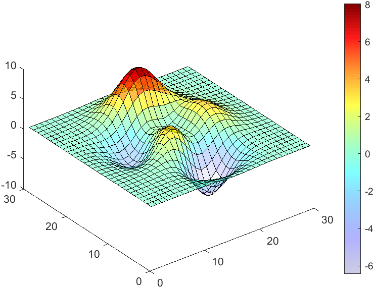
The code will work if the plot have AlphaData property
data = peaks(30);
AData = rescale(data, .2, 1);
surface(data, 'FaceAlpha','flat','AlphaData',AData);
colormap(jet(100));
ax = gca;
ax.DataAspectRatio = [1,1,1];
ax.TickDir = 'out';
ax.Box = 'off';
view(3)
CBarHdl = colorbar;
pause(1e-16)
CData = CBarHdl.Face.Texture.CData;
ALim = [min(min(AData)), max(max(AData))];
CData(4,:) = uint8(255.*rescale(1:size(CData, 2), ALim(1), ALim(2)));
warning off
CBarHdl.Face.ColorType = 'TrueColorAlpha';
VertexData = CBarHdl.Face.VertexData;
tY = repmat((1:size(CData,2))./size(CData,2), [4,1]);
tY1 = tY(:).'; tY2 = tY - tY(1,1); tY2(3:4,:) = 0; tY2 = tY2(:).';
tM1 = [tY1.*0 + 1; tY1; tY1.*0 + 1];
tM2 = [tY1.*0; tY2; tY1.*0];
CBarHdl.Face.VertexData = repmat(VertexData, [1,size(CData,2)]).*tM1 + tM2;
CBarHdl.Face.ColorData = reshape(repmat(CData, [4,1]), 4, []);

Many MATLAB enthusiasts come Cody to sharpen their skills, face new challenges, and engage in friendly competition. We firmly believe that learning from peers is one of the most effective ways to grow.
With this in mind, the Cody team is thrilled to unveil a new feature aimed at enriching your learning journey: the Cody Discussion Channel. This space is designed for sharing expertise, acquiring new skills, and fostering connections within our community.
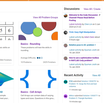
On the Cody homepage, you'll now notice a Discussions section, prominently displaying the four most recent posts. For those eager to contribute, we encourage you to familiarize yourself with our posting guidelines before creating a new post. This will help maintain a constructive and valuable exchange of ideas for everyone involved.
Together, let's create an environment where every member feels empowered to share, learn, and connect.
There are a host of problems on Cody that require manipulation of the digits of a number. Examples include summing the digits of a number, separating the number into its powers, and adding very large numbers together.
If you haven't come across this trick yet, you might want to write it down (or save it electronically):
digits = num2str(4207) - '0'
That code results in the following:
digits =
4 2 0 7
Now, summing the digits of the number is easy:
sum(digits)
ans =
13
Hello and a warm welcome to everyone! We're excited to have you in the Cody Discussion Channel. To ensure the best possible experience for everyone, it's important to understand the types of content that are most suitable for this channel.
Content that belongs in the Cody Discussion Channel:
- Tips & tricks: Discuss strategies for solving Cody problems that you've found effective.
- Ideas or suggestions for improvement: Have thoughts on how to make Cody better? We'd love to hear them.
- Issues: Encountering difficulties or bugs with Cody? Let us know so we can address them.
- Requests for guidance: Stuck on a Cody problem? Ask for advice or hints, but make sure to show your efforts in attempting to solve the problem first.
- General discussions: Anything else related to Cody that doesn't fit into the above categories.
Content that does not belong in the Cody Discussion Channel:
- Comments on specific Cody problems: Examples include unclear problem descriptions or incorrect testing suites.
- Comments on specific Cody solutions: For example, you find a solution creative or helpful.
Please direct such comments to the Comments section on the problem or solution page itself.
We hope the Cody discussion channel becomes a vibrant space for sharing expertise, learning new skills, and connecting with others.
One of the starter prompts is about rolling two six-sided dice and plot the results. As a hobby, I create my own board games. I was able to use the dice rolling prompt to show how a simple roll and move game would work. That was a great surprise!
How to leave feedback on a doc page
Leaving feedback is a two-step process. At the bottom of most pages in the MATLAB documentation is a star rating.
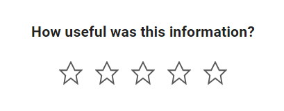
Start by selecting a star that best answers the question. After selecting a star rating, an edit box appears where you can offer specific feedback.
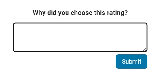
When you press "Submit" you'll see the confirmation dialog below. You cannot go back and edit your content, although you can refresh the page to go through that process again.

Tips on leaving feedback
- Be productive. The reader should clearly understand what action you'd like to see, what was unclear, what you think needs work, or what areas were really helpful.
- Positive feedback is also helpful. By nature, feedback often focuses on suggestions for changes but it also helps to know what was clear and what worked well.
- Point to specific areas of the page. This helps the reader to narrow the focus of the page to the area described by your feedback.
What happens to that feedback?
Before working at MathWorks I often left feedback on documentation pages but I never knew what happens after that. One day in 2021 I shared my speculation on the process:
> That feedback is received by MathWorks Gnomes which are never seen nor heard but visit the MathWorks documentation team at night while they are sleeping and whisper selected suggestions into their ears to manipulate their dreams. Occassionally this causes them to wake up with a Eureka moment that leads to changes in the documentation.

I'd like to let you in on the secret which is much less fanciful. Feedback left in the star rating and edit box are collected and periodically reviewed by the doc writers who look for trends on highly trafficked pages and finer grain feedback on less visited pages. Your feedback is important and often results in improvements.
Hello MATLAB Community!
We've had an exciting few weeks filled with insightful discussions, innovative tools, and engaging blog posts from our vibrant community. Here's a highlight of some noteworthy contributions that have sparked interest and inspired us all. Let's dive in!
Interesting Questions
Cindyawati explores the intriguing concept of interrupting continuous data in differential equations to study the effects of drug interventions in disease models. A thought-provoking question that bridges mathematics and medical research.
Pedro delves into the application of Linear Quadratic Regulator (LQR) for error dynamics and setpoint tracking, offering insights into control systems and their real-world implications.
Popular Discussions
Chen Lin shares an engaging interview with Zhaoxu Liu, shedding light on the creative processes behind some of the most innovative MATLAB contest entries of 2023. A must-read for anyone looking for inspiration!
Zhaoxu Liu, also known as slanderer, updates the community with the latest version of the MATLAB Plot Cheat Sheet. This resource is invaluable for anyone looking to enhance their data visualization skills.
From File Exchange
Giorgio introduces a toolbox for frequency estimation, making it simpler for users to import signals directly from the MATLAB workspace. A significant contribution for signal processing enthusiasts.
From the Blogs
Cleve Moler revisits a classic program for predicting future trends based on census data, offering a fascinating glimpse into the evolution of computational forecasting.
Boost Your App Design Efficiency – Effortless Component Swapping & Labeling in App Designer by Adam Danz
With contributions from Dinesh Kavalakuntla, Adam presents an insightful guide on improving app design workflows in MATLAB App Designer, focusing on component swapping and labeling.
We're incredibly proud of the diverse and innovative contributions our community members make every day. Each post, discussion, and tool not only enriches our knowledge but also inspires others to explore and create. Let's continue to support and learn from each other as we advance in our MATLAB journey.
Happy Coding!
quick / easy
21%
themed / in a group
21%
challenge (e.g., banned functions)
14%
puzzle / game
15%
educational
27%
other (comment below)
3%
111 个投票
A colleague said that you can search the Help Center using the phrase 'Introduced in' followed by a release version. Such as, 'Introduced in R2022a'. Doing this yeilds search results specific for that release.
Seems pretty handy so I thought I'd share.
Bringing the beauty of MathWorks Natick's tulips to life through code!
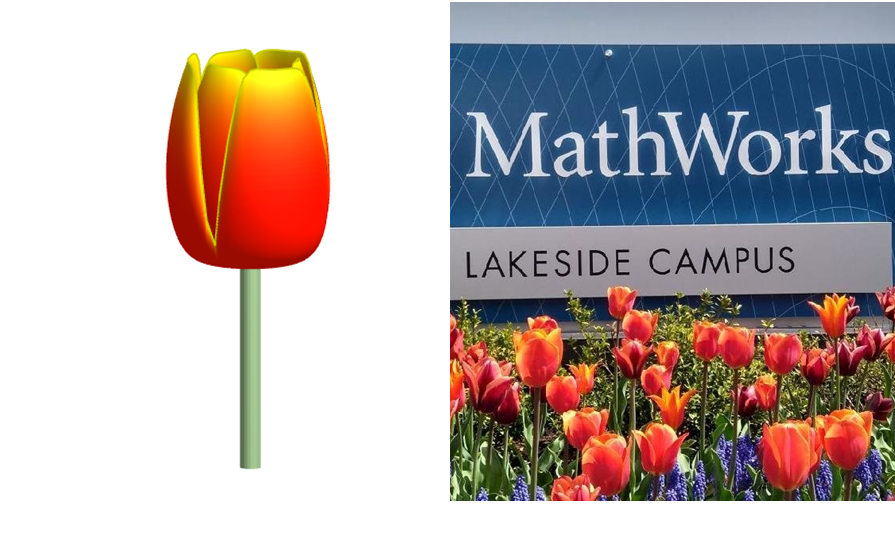
Remix challenge: create and share with us your new breeds of MATLAB tulips!
RGB triplet [0,1]
9%
RGB triplet [0,255]
12%
Hexadecimal Color Code
13%
Indexed color
16%
Truecolor array
37%
Equally unfamiliar with all-above
13%
2703 个投票
A high school student called for help with this physics problem:
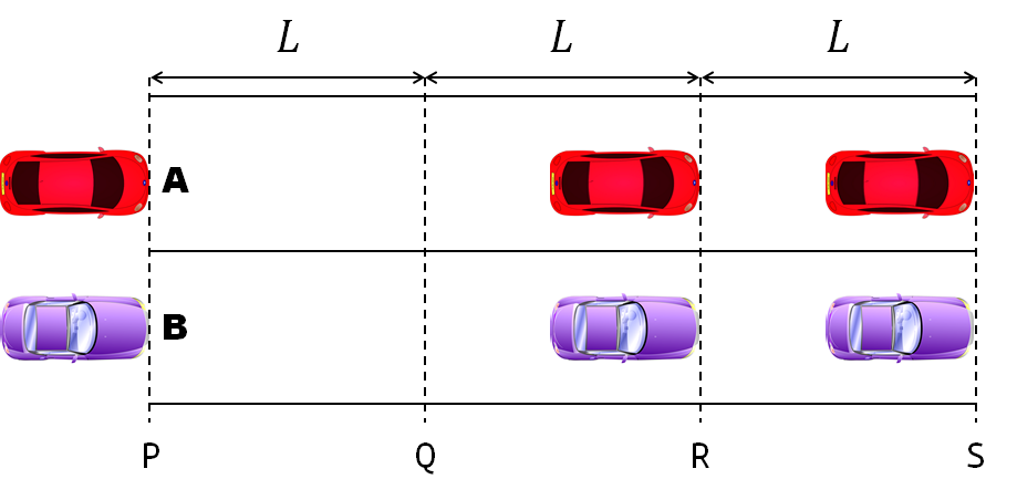
- Car A moves with constant velocity v.
- Car B starts to move when Car A passes through the point P.
- Car B undergoes...
- uniform acc. motion from P to Q.
- uniform velocity motion from Q to R.
- uniform acc. motion from R to S.
- Car A and B pass through the point R simultaneously.
- Car A and B arrive at the point S simultaneously.
Q1. When car A passes the point Q, which is moving faster?
Q2. Solve the time duration for car B to move from P to Q using L and v.
Q3. Magnitude of acc. of car B from P to Q, and from R to S: which is bigger?
Well, it can be solved with a series of tedious equations. But... how about this?
Code below:
%% get images and prepare stuffs
figure(WindowStyle="docked"),
ax1 = subplot(2,1,1);
hold on, box on
ax1.XTick = [];
ax1.YTick = [];
A = plot(0, 1, 'ro', MarkerSize=10, MarkerFaceColor='r');
B = plot(0, 0, 'bo', MarkerSize=10, MarkerFaceColor='b');
[carA, ~, alphaA] = imread('https://cdn.pixabay.com/photo/2013/07/12/11/58/car-145008_960_720.png');
[carB, ~, alphaB] = imread('https://cdn.pixabay.com/photo/2014/04/03/10/54/car-311712_960_720.png');
carA = imrotate(imresize(carA, 0.1), -90);
carB = imrotate(imresize(carB, 0.1), 180);
alphaA = imrotate(imresize(alphaA, 0.1), -90);
alphaB = imrotate(imresize(alphaB, 0.1), 180);
carA = imagesc(carA, AlphaData=alphaA, XData=[-0.1, 0.1], YData=[0.9, 1.1]);
carB = imagesc(carB, AlphaData=alphaB, XData=[-0.1, 0.1], YData=[-0.1, 0.1]);
txtA = text(0, 0.85, 'A', FontSize=12);
txtB = text(0, 0.17, 'B', FontSize=12);
yline(1, 'r--')
yline(0, 'b--')
xline(1, 'k--')
xline(2, 'k--')
text(1, -0.2, 'Q', FontSize=20, HorizontalAlignment='center')
text(2, -0.2, 'R', FontSize=20, HorizontalAlignment='center')
% legend('A', 'B') % this make the animation slow. why?
xlim([0, 3])
ylim([-.3, 1.3])
%% axes2: plots velocity graph
ax2 = subplot(2,1,2);
box on, hold on
xlabel('t'), ylabel('v')
vA = plot(0, 1, 'r.-');
vB = plot(0, 0, 'b.-');
xline(1, 'k--')
xline(2, 'k--')
xlim([0, 3])
ylim([-.3, 1.8])
p1 = patch([0, 0, 0, 0], [0, 1, 1, 0], [248, 209, 188]/255, ...
EdgeColor = 'none', ...
FaceAlpha = 0.3);
%% solution
v = 1; % car A moves with constant speed.
L = 1; % distances of P-Q, Q-R, R-S
% acc. of car B for three intervals
a(1) = 9*v^2/8/L;
a(2) = 0;
a(3) = -1;
t_BatQ = sqrt(2*L/a(1)); % time when car B arrives at Q
v_B2 = a(1) * t_BatQ; % speed of car B between Q-R
%% patches for velocity graph
p2 = patch([t_BatQ, t_BatQ, t_BatQ, t_BatQ], [1, 1, v_B2, v_B2], ...
[248, 209, 188]/255, ...
EdgeColor = 'none', ...
FaceAlpha = 0.3);
p3 = patch([2, 2, 2, 2], [1, v_B2, v_B2, 1], [194, 234, 179]/255, ...
EdgeColor = 'none', ...
FaceAlpha = 0.3);
%% animation
tt = linspace(0, 3, 2000);
for t = tt
A.XData = v * t;
vA.XData = [vA.XData, t];
vA.YData = [vA.YData, 1];
if t < t_BatQ
B.XData = 1/2 * a(1) * t^2;
vB.XData = [vB.XData, t];
vB.YData = [vB.YData, a(1) * t];
p1.XData = [0, t, t, 0];
p1.YData = [0, vB.YData(end), 1, 1];
elseif t >= t_BatQ && t < 2
B.XData = L + (t - t_BatQ) * v_B2;
vB.XData = [vB.XData, t];
vB.YData = [vB.YData, v_B2];
p2.XData = [t_BatQ, t, t, t_BatQ];
p2.YData = [1, 1, vB.YData(end), vB.YData(end)];
else
B.XData = 2*L + v_B2 * (t - 2) + 1/2 * a(3) * (t-2)^2;
vB.XData = [vB.XData, t];
vB.YData = [vB.YData, v_B2 + a(3) * (t - 2)];
p3.XData = [2, t, t, 2];
p3.YData = [1, 1, vB.YData(end), v_B2];
end
txtA.Position(1) = A.XData(end);
txtB.Position(1) = B.XData(end);
carA.XData = A.XData(end) + [-.1, .1];
carB.XData = B.XData(end) + [-.1, .1];
drawnow
end
is there any sites available online free ai course learning except: coursera.org
Northern lights captured from this weekend at MathWorks campus ✨
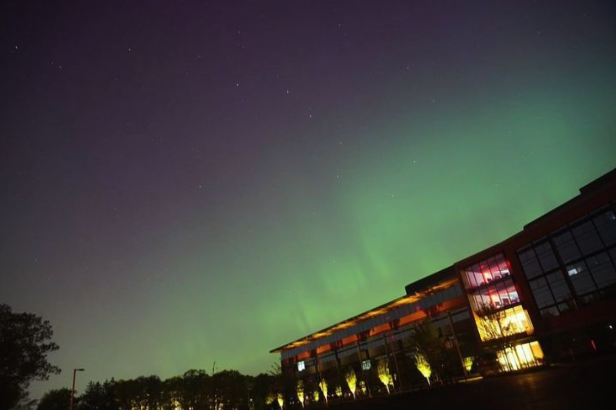
Did you get a chance to see lights and take some photos?
From Alpha Vantage's website: API Documentation | Alpha Vantage
Try using the built-in Matlab function webread(URL)... for example:
% copy a URL from the examples on the site
URL = 'https://www.alphavantage.co/query?function=TIME_SERIES_DAILY&symbol=IBM&apikey=demo'
% or use the pattern to create one
tickers = [{'IBM'} {'SPY'} {'DJI'} {'QQQ'}]; i = 1;
URL = ...
['https://www.alphavantage.co/query?function=TIME_SERIES_DAILY_ADJUSTED&outputsize=full&symbol=', ...
+ tickers{i}, ...
+ '&apikey=***Put Your API Key here***'];
X = webread(URL);
You can access any of the data available on the site as per the Alpha Vantage documentation using these two lines of code but with different designations for the requested data as per the documentation.
It's fun!
您也可以从以下列表中选择网站:
美洲
- América Latina (Español)
- Canada (English)
- United States (English)
欧洲
- Belgium (English)
- Denmark (English)
- Deutschland (Deutsch)
- España (Español)
- Finland (English)
- France (Français)
- Ireland (English)
- Italia (Italiano)
- Luxembourg (English)
- Netherlands (English)
- Norway (English)
- Österreich (Deutsch)
- Portugal (English)
- Sweden (English)
- Switzerland
- United Kingdom(English)
亚太
- Australia (English)
- India (English)
- New Zealand (English)
- 中国
- 日本Japanese (日本語)
- 한국Korean (한국어)