主要内容
搜索
I created an ellipse visualizer in #MATLAB using App Designer! To read more about it, and how it ties to the recent total solar eclipse, check out my latest blog post:
Github Repo of the app (you can open it on MATLAB Online!):
I'm excited to share some valuable resources that I've found to be incredibly helpful for anyone looking to enhance their MATLAB skills. Whether you're just starting out, studying as a student, or are a seasoned professional, these guides and books offer a wealth of information to aid in your learning journey.
These materials are freely available and can be a great addition to your learning resources. They cover a wide range of topics and are designed to help users at all levels to improve their proficiency in MATLAB.
Happy learning and I hope you find these resources as useful as I have!
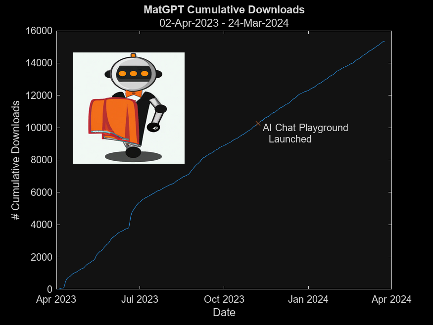
MatGPT was launched on March 22, 2023 and I am amazed at how many times it has been downloaded since then - close to 16,000 downloads in one year. When AI Chat Playground came out on MATLAB Central, I thought surely that people will stop using MatGPT. Boy I was wrong.

In early 2023 I was playing with the new shiny toy called ChatGPT like everyone else but instead of having it tell me jokes or haiku, I wanted to know how I can use it on MATLAB, and I started collecting the prompts that worked. Someone suggested I should turn that into an app, and MatGPT was born with help from other colleagues.
Here is the question - what should I do with it now? Some people suggested I could add other LLMs like Gemini or Claude, but I am more interested in learning how people actually use it.
If you are a MatGPT user, do you mind sharing how you use the app?
Let S be the closed surface composed of the hemisphere  and the base
  Let
Let  be the electric field defined by
  . Find the electric flux through S. (Hint: Divide S into two parts and calculate
  ).
).
% Define the limits of integration for the hemisphere S1
theta_lim = [-pi/2, pi/2];
phi_lim = [0, pi/2];
% Perform the double integration over the spherical surface of the hemisphere S1
% Define the electric flux function for the hemisphere S1
flux_function_S1 = @(theta, phi) 2 * sin(phi);
electric_flux_S1 = integral2(flux_function_S1, theta_lim(1), theta_lim(2), phi_lim(1), phi_lim(2));
% For the base of the hemisphere S2, the electric flux is 0 since the electric
% field has no z-component at the base
electric_flux_S2 = 0;
% Calculate the total electric flux through the closed surface S
total_electric_flux = electric_flux_S1 + electric_flux_S2;
% Display the flux calculations
disp(['Electric flux through the hemisphere S1: ', num2str(electric_flux_S1)]);
disp(['Electric flux through the base of the hemisphere S2: ', num2str(electric_flux_S2)]);
disp(['Total electric flux through the closed surface S: ', num2str(total_electric_flux)]);
% Parameters for the plot
radius = 1; % Radius of the hemisphere
% Create a meshgrid for theta and phi for the plot
[theta, phi] = meshgrid(linspace(theta_lim(1), theta_lim(2), 20), linspace(phi_lim(1), phi_lim(2), 20));
% Calculate Cartesian coordinates for the points on the hemisphere
x = radius * sin(phi) .* cos(theta);
y = radius * sin(phi) .* sin(theta);
z = radius * cos(phi);
% Define the electric field components
Ex = 2 * x;
Ey = 2 * y;
Ez = 2 * z;
% Plot the hemisphere
figure;
surf(x, y, z, 'FaceAlpha', 0.5, 'EdgeColor', 'none');
hold on;
% Plot the electric field vectors
quiver3(x, y, z, Ex, Ey, Ez, 'r');
% Plot the base of the hemisphere
[x_base, y_base] = meshgrid(linspace(-radius, radius, 20), linspace(-radius, radius, 20));
z_base = zeros(size(x_base));
surf(x_base, y_base, z_base, 'FaceColor', 'cyan', 'FaceAlpha', 0.3);
% Additional plot settings
colormap('cool');
axis equal;
grid on;
xlabel('X');
ylabel('Y');
zlabel('Z');
title('Hemisphere and Electric Field');

I feel like no one at UC San Diego knows this page, let alone this server, is still live. For the younger generation, this is what the whole internet used to look like :)

In short: support varying color in at least the plot, plot3, fplot, and fplot3 functions.
This has been a thing that's come up quite a few times, and includes questions/requests by users, workarounds by the community, and workarounds presented by MathWorks -- examples of each below. It's a feature that exists in Python's Matplotlib library and Sympy. Anyways, given that there are myriads of workarounds, it appears to be one of the most common requests for Matlab plots (Matlab's plotting is, IMO, one of the best features of the product), the request precedes the 21st century, and competitive tools provide the functionality, it would seem to me that this might be the next great feature for Matlab plotting.
I'm curious to get the rest of the community's thoughts... what's everyone else think about this?
---
User questions/requests
- https://www.mathworks.com/matlabcentral/answers/480389-colored-line-plot-according-to-a-third-variable
- https://www.mathworks.com/matlabcentral/answers/2092641-how-to-solve-a-problem-with-the-generation-of-multiple-colored-segments-on-one-line-in-matlab-plot
- https://www.mathworks.com/matlabcentral/answers/5042-how-do-i-vary-color-along-a-2d-line
- https://www.mathworks.com/matlabcentral/answers/1917650-how-to-plot-a-trajectory-with-varying-colour
- https://www.mathworks.com/matlabcentral/answers/1917650-how-to-plot-a-trajectory-with-varying-colour
- https://www.mathworks.com/matlabcentral/answers/511523-how-to-create-plot3-varying-color-figure
- https://www.mathworks.com/matlabcentral/answers/393810-multiple-colours-in-a-trajectory-plot
- https://www.mathworks.com/matlabcentral/answers/523135-creating-a-rainbow-colour-plot-trajectory
- https://www.mathworks.com/matlabcentral/answers/469929-how-to-vary-the-color-of-a-dynamic-line
- https://www.mathworks.com/matlabcentral/answers/585011-how-could-i-adjust-the-color-of-multiple-lines-within-a-graph-without-using-the-default-matlab-colo
- https://www.mathworks.com/matlabcentral/answers/517177-how-to-interpolate-color-along-a-curve-with-specific-colors
- https://www.mathworks.com/matlabcentral/answers/281645-variate-color-depending-on-the-y-value-in-plot
- https://www.mathworks.com/matlabcentral/answers/439176-how-do-i-vary-the-color-along-a-line-in-polar-coordinates
- https://www.mathworks.com/matlabcentral/answers/1849193-creating-rainbow-coloured-plots-in-3d
- https://groups.google.com/g/comp.soft-sys.matlab/c/cLgjSeEC15I?hl=en&pli=1 (a question asked in 1999!)
- ... the list goes on, and on, and on...
User-provided workarounds
- https://undocumentedmatlab.com/articles/plot-line-transparency-and-color-gradient
- https://www.mathworks.com/matlabcentral/fileexchange/19476-colored-line-or-scatter-plot
- https://www.mathworks.com/matlabcentral/fileexchange/23566-3d-colored-line-plot
- https://www.mathworks.com/matlabcentral/fileexchange/30423-conditionally-colored-line-plot
- https://www.mathworks.com/matlabcentral/fileexchange/14677-cline
- https://www.mathworks.com/matlabcentral/fileexchange/8597-plot-3d-color-line
- https://www.mathworks.com/matlabcentral/fileexchange/39972-colormapline-color-changing-2d-or-3d-line
- https://www.mathworks.com/matlabcentral/fileexchange/37725-conditionally-colored-plot-ccplot
- https://www.mathworks.com/matlabcentral/fileexchange/11611-linear-2d-plot-with-rainbow-color
- https://www.mathworks.com/matlabcentral/fileexchange/26692-color_line
- https://www.mathworks.com/matlabcentral/fileexchange/32911-plot3rgb
- And perhaps more?
MathWorks-provided workarounds
- https://www.mathworks.com/videos/coloring-a-line-based-on-height-gradient-or-some-other-value-in-matlab-97128.html
- https://www.mathworks.com/videos/making-a-multi-color-line-in-matlab-97127.html
- https://www.mathworks.com/matlabcentral/fileexchange/95663-color-trajectory-plot (contributed by a MathWorks staff member)
- And perhaps more?
colored Line plot according to a third variable
Hello, I already asked this question before but it is really important to have an answer since the last answer i got wasn't helpful. i will post the whole code: "hold on load(Filename.mat') ...
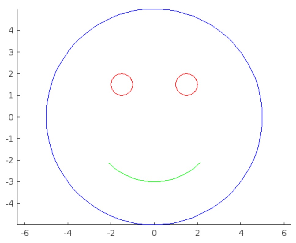
I was in a meeting the other day and a coworker shared a smiley face they created using the AI Chat Playground. The image looked something like this:

And I suspect the prompt they used was something like this:
"Create a smiley face"
I imagine this output wasn't what my coworker had expected so he was left thinking that this was as good as it gets without manually editing the code, and that the AI Chat Playground couldn't do any better.
I thought I could get a better result using the Playground so I tried a more detailed prompt using a multi-step technique like this:
"Follow these instructions:
- Create code that plots a circle
- Create two smaller circles as eyes within the first circle
- Create an arc that looks like a smile in the lower part of the first circle"
The output of this prompt was better in my opinion.

These queries/prompts are examples of 'zero-shot' prompts, the expectation being a good result with just one query. As opposed to a back-and-forth chat session working towards a desired outcome.
I wonder how many attempts everyone tries before they decide they can't anything more from the AI/LLM. There are times I'll send dozens of chat queries if I feel like I'm getting close to my goal, while other times I'll try just one or two. One thing I always find useful is seeing how others interact with AI models, which is what inspired me to share this.
Does anyone have examples of techniques that work well? I find multi-step instructions often produces good results.
Although, I think I will only get to see a partial eclipse (April 8th!) from where I am at in the U.S. I will always have MATLAB to make my own solar eclipse. Just as good as the real thing.
Code (found on the @MATLAB instagram)
a=716;
v=255;
X=linspace(-10,10,a);
[~,r]=cart2pol(X,X');
colormap(gray.*[1 .78 .3]);
[t,g]=cart2pol(X+2.6,X'+1.4);
image(rescale(-1*(2*sin(t*10)+60*g.^.2),0,v))
hold on
h=exp(-(r-3)).*abs(ifft2(r.^-1.8.*cos(7*rand(a))));
h(r<3)=0;
image(v*ones(a),'AlphaData',rescale(h,0,1))
camva(3.8)

One of the privileges of working at MathWorks is that I get to hang out with some really amazing people. Steve Eddins, of ‘Steve on Image Processing’ fame is one of those people. He recently announced his retirement and before his final day, I got the chance to interview him. See what he had to say over at The MATLAB Blog The Steve Eddins Interview: 30 years of MathWorking
Before we begin, you will need to make sure you have 'sir_age_model.m' installed. Once you've downloaded this folder into your working directory, which can be located at your current folder. If you can see this file in your current folder, then it's safe to use it. If you choose to use MATLAB online or MATLAB Mobile, you may upload this to your MATLAB Drive.
This is the code for the SIR model stratified into 2 age groups (children and adults). For a detailed explanation of how to derive the force of infection by age group.
% Main script to run the SIR model simulation
% Initial state values
initial_state_values = [200000; 1; 0; 800000; 0; 0]; % [S1; I1; R1; S2; I2; R2]
% Parameters
parameters = [0.05; 7; 6; 1; 10; 1/5]; % [b; c_11; c_12; c_21; c_22; gamma]
% Time span for the simulation (3 months, with daily steps)
tspan = [0 90];
% Solve the ODE
[t, y] = ode45(@(t, y) sir_age_model(t, y, parameters), tspan, initial_state_values);
% Plotting the results
plot(t, y);
xlabel('Time (days)');
ylabel('Number of people');
legend('S1', 'I1', 'R1', 'S2', 'I2', 'R2');
title('SIR Model with Age Structure');

What was the cumulative incidence of infection during this epidemic? What proportion of those infections occurred in children?
In the SIR model, the cumulative incidence of infection is simply the decline in susceptibility.
% Assuming 'y' contains the simulation results from the ode45 function
% and 't' contains the time points
% Total cumulative incidence
total_cumulative_incidence = (y(1,1) - y(end,1)) + (y(1,4) - y(end,4));
fprintf('Total cumulative incidence: %f\n', total_cumulative_incidence);
% Cumulative incidence in children
cumulative_incidence_children = (y(1,1) - y(end,1));
% Proportion of infections in children
proportion_infections_children = cumulative_incidence_children / total_cumulative_incidence;
fprintf('Proportion of infections in children: %f\n', proportion_infections_children);
927,447 people became infected during this epidemic, 20.5% of which were children.
Which age group was most affected by the epidemic?
To answer this, we can calculate the proportion of children and adults that became infected.
% Assuming 'y' contains the simulation results from the ode45 function
% and 't' contains the time points
% Proportion of children that became infected
initial_children = 200000; % initial number of susceptible children
final_susceptible_children = y(end,1); % final number of susceptible children
proportion_infected_children = (initial_children - final_susceptible_children) / initial_children;
fprintf('Proportion of children that became infected: %f\n', proportion_infected_children);
% Proportion of adults that became infected
initial_adults = 800000; % initial number of susceptible adults
final_susceptible_adults = y(end,4); % final number of susceptible adults
proportion_infected_adults = (initial_adults - final_susceptible_adults) / initial_adults;
fprintf('Proportion of adults that became infected: %f\n', proportion_infected_adults);
Throughout this epidemic, 95% of all children and 92% of all adults were infected. Children were therefore slightly more affected in proportion to their population size, even though the majority of infections occurred in adults.
Are you going to be in the path of totality? How can you predict, track, and simulate the solar eclipse using MATLAB?
I would like to propose the creation of MATLAB EduHub, a dedicated channel within the MathWorks community where educators, students, and professionals can share and access a wealth of educational material that utilizes MATLAB. This platform would act as a central repository for articles, teaching notes, and interactive learning modules that integrate MATLAB into the teaching and learning of various scientific fields.
Key Features:
1. Resource Sharing: Users will be able to upload and share their own educational materials, such as articles, tutorials, code snippets, and datasets.
2. Categorization and Search: Materials can be categorized for easy searching by subject area, difficulty level, and MATLAB version..
3. Community Engagement: Features for comments, ratings, and discussions to encourage community interaction.
4. Support for Educators: Special sections for educators to share teaching materials and track engagement.
Benefits:
- Enhanced Educational Experience: The platform will enrich the learning experience through access to quality materials.
- Collaboration and Networking: It will promote collaboration and networking within the MATLAB community.
- Accessibility of Resources: It will make educational materials available to a wider audience.
By establishing MATLAB EduHub, I propose a space where knowledge and experience can be freely shared, enhancing the educational process and the MATLAB community as a whole.
In one line of MATLAB code, compute how far you can see at the seashore. In otherwords, how far away is the horizon from your eyes? You can assume you know your height and the diameter or radius of the earth.


