搜索
Hi,
I need to know how to resolve EDO System with MATLAB. The system has this structure:
A*x̄' + B*x̄ + C = 0
A, B are square matrix with constant coefficients. Example: A = [a b; c d]; and B = [e f; g h];
C is the constant vector transposed. Example: C = [i j]';
x̄ is the vector transposed of the variables/functions I need to find. Example: x̄ = [x1 x2]';
x̄' is the vector transposed of the derivative of the variables/functions I need to find. Example: x̄' = [dx1/dt dx2/dt]';
The example is made for a EDO System of 2 differential equations. But It would be interesting if MATLAB could resolve a n x n matrix.
Any suggestion?
Iam doing the project to find machining time for the cnc by creating a MATLAB Program ,I have G and M code in text file and the program should accept below points
- Read each line from the file.
- Extract the distance from G-code commands and the feedrate for each line.
- Calculate the time for each movement using the formula: time = distance / feedrate.
- Sum the times for all lines to get the total machining time.
Conditions:
G01 commands represent linear movements, so we calculate the distance directly.
G02 and G03 commands denote circular interpolation (clockwise and counterclockwise arcs, respectively). For these, compute the distance traveled along the arc.
For example, this below line is circular interpolation from G and M code Text file.
N1754 G03 X72.704 I10.704 J28.773 F2198.429
Could any one help me what formula should I use to get tool path for circular interpolation and linear interpolation to extract the distance.
Imagine that the earth is a perfect sphere with a radius of 6371000 meters and there is a rope tightly wrapped around the equator. With one line of MATLAB code determine how much the rope will be lifted above the surface if you cut it and insert a 1 meter segment of rope into it (and then expand the whole rope back into a circle again, of course).
Hello,
I am using BEAR TOOLBOX to obtain impulse response function of outcome variable to the 25 basis point monetary policy shock. The problem is there is no option in App of BEAR toolbox. how can i do it . please suggest
Hello everybody. I'm using Newton's method to solve a liner equation whose solution should be in [0 1]. Unfortunately, the coe I'm using gives NaN as a result for a specific combination of parameters and I would like to understand if I can improve the code I wrote for my Newton's method. In the specific case I'm considering, I reach the maximum iterations even if the tolerance is very low.
function [x,n,ier] = newton(f,fd,x0,nmax,tol)
% Newton's method for non-linear equations
ier = 0;
for n = 1:nmax
x = x0-f(x0)/fd(x0);
if abs(x-x0) <= tol
ier = 1;
break
end
x0 = x;
end
% % % % Script for solving NaN
mNAN= 16.1;
lNAN= 10^-4;
f= @(x) mNAN*x+lNAN*exp(mNAN*x)-lNAN*exp(mNAN);
Fd= @(x) mNAN*(1+lNAN*exp(mNAN*x));
tolNaN=10^-1;
nmax=10^8;
AB0 = 0.5;
[amNAN,nNAN,ierNAN]=newton(f,Fd,AB0,nmax,tolNaN);
amNAN
Llimit=f(0)
Ulimit=f(1)
fplot(@(x) mNAN*x+lNAN*exp(mNAN*x)-lNAN*exp(mNAN),[0 1.1])
Swimming, diving
16%
Other water-based sport
4%
Gymnastics
20%
Other indoor arena sport
15%
track, field
24%
Other outdoor sport
21%
346 个投票
Hello, MATLAB enthusiasts! 🌟
Over the past few weeks, our community has been buzzing with insightful questions, vibrant discussions, and innovative ideas. Whether you're a seasoned expert or a curious beginner, there's something here for everyone to learn and enjoy. Let's take a moment to highlight some of the standout contributions that have sparked interest and inspired many. Dive in and see how you can join the conversation or find solutions to your own challenges!
Interesting Questions
How can i edit my code which works on r2014b version at work but not on my personal r2024a version? by Oluwadamilola Oke
Oluwadamilola Oke is seeking assistance with a MATLAB code that works on version r2014b but encounters errors on version r2024a. The issue seems to be related to file location or the use of specific commands like movefile. If you have experience with these versions of MATLAB, your expertise could be invaluable.
Yohay has been working on a simulation to measure particle speed and fit it to the Maxwell-Boltzmann distribution. However, the fit isn't aligning perfectly with the data. Yohay has shared the code and histogram data for community members to review and provide suggestions.
Alessandro Livi is toggling between C++ for Arduino Pico and MATLAB App Designer. They suggest an enhancement where typing // for comments in MATLAB automatically converts to %. This small feature could improve the workflow for many users who switch between programming languages.
Popular Discussions
Athanasios Paraskevopoulos has started an engaging discussion on Gabriel's Horn, a shape with infinite surface area but finite volume. The conversation delves into the mathematical intricacies and integral calculations required to understand this paradoxical shape.
Honzik has brought up an interesting topic about custom fonts for MATLAB. While popular coding fonts handle characters like 0 and O well, they often fail to distinguish between different types of brackets. Honzik suggests that MathWorks could develop a custom font optimized for MATLAB syntax to reduce coding errors.
From the Blogs
Guy Rouleau addresses a common error in Simulink models: "Derivative of state '1' in block 'X/Y/Integrator' at time 0.55 is not finite." The blog post explores various tools and methods to diagnose and resolve this issue, making it a valuable read for anyone facing similar challenges.
Guest writer Gianluca Carnielli, featured by Adam Danz, shares insights on creating time-sensitive animations using MATLAB. The article covers controlling the motion of multiple animated objects, organizing data with timetables, and simplifying animations with the retime function. This is a must-read for anyone interested in scientific animations.
Feel free to check out these fascinating contributions and join the discussions! Your input and expertise can make a significant difference in our community.
hello i found the following tools helpful to write matlab programs. copilot.microsoft.com chatgpt.com/gpts gemini.google.com and ai.meta.com. thanks a lot and best wishes.
Check out the LLMs with MATLAB project on File Exchange to access Large Language Models from MATLAB.
Along with the latest support for GPT-4o mini, you can use LLMs with MATLAB to generate images, categorize data, and provide semantic analyis.
function ans = your_fcn_name(n)
n;
j=sum(1:n);
a=zeros(1,j);
for i=1:n
a(1,((sum(1:(i-1))+1)):(sum(1:(i-1))+i))=i.*ones(1,i);
end
disp
I am trying to earn my Intro to MATLAB badge in Cody, but I cannot click the Roll the Dice! problem. It simply is not letting me click it, therefore I cannot earn my badge. Does anyone know who I should contact or what to do?
I define the class in matlab as:
classdef Myclass
properties
Content
end
methods
function obj = Myclass(content)
obj.Content = content;
end
function disp(obj)
A = symmatrix('A(1/3,[0,0,1])');
disp(A);
end
end
end
When we run this class in live editor return 'A(1/3,[0,0,1])' rather than latex form.
Myclass(1)
% return 'A(1/3,[0,0,1])'
A = symmatrix('A(1/3,[0,0,1])');
% return latrx form A(1/3,[0,0,1])
Something that had bothered me ever since I became an FEA analyst (2012) was the apparent inability of the "camera" in Matlab's 3D plot to function like the "cameras" in CAD/CAE packages.
For instance, load the ForearmLink.stl model that ships with the PDE Toolbox in Matlab and ParaView and try rotating the model.
clear
close all
gm = importGeometry( "ForearmLink.stl" );
pdegplot(gm)
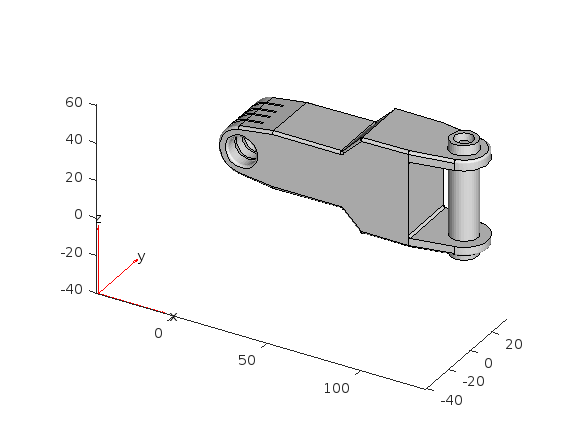
Things to observe:
- Note that I cant seem to rotate continuously around the x-axis. It appears to only support rotations from [0, 360] as opposed to [-inf, inf]. So, for example, if I'm looking in the Y+ direction and rotate around X so that I'm looking at the Z- direction, and then want to look in the Y- direction, I can't simply keep rotating around the X axis... instead have to rotate 180 degrees around the Z axis and then around the X axis. I'm not aware of any data visualization applications (e.g., ParaView, VisIt, EnSight) or CAD/CAE tools with such an interaction.
- Note that at the 50 second mark, I set a view in ParaView: looking in the [X-, Y-, Z-] direction with Y+ up. Try as I might in Matlab, I'm unable to achieve that same view perspective.
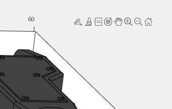
Today I discovered that if one turns on the Camera Toolbar from the View menubar, then clicks the Orbit Camera icon, then the No Principal Axis icon:
That then it acts in the manner I've long desired. Oh, and also, for the interested, it is programmatically available: https://www.mathworks.com/help/matlab/ref/cameratoolbar.html
I might humbly propose this mode either be made more discoverable, similar to the little interaction widgets that pop up in figures:
Or maybe use the middle-mouse button to temporarily use this mode (a mouse setting in, e.g., Abaqus/CAE).
I've noticed is that the highly rated fonts for coding (e.g. Fira Code, Inconsolata, etc.) seem to overlook one issue that is key for coding in Matlab. While these fonts make 0 and O, as well as the 1 and l easily distinguishable, the brackets are not. Quite often the curly bracket looks similar to the curved bracket, which can lead to mistakes when coding or reviewing code.
So I was thinking: Could Mathworks put together a team to review good programming fonts, and come up with their own custom font designed specifically and optimized for Matlab syntax?
could you explain me how to calculate the gain values for different types of controllers (Conventional Sliding Mode Control, Third Order Sliding Mode Control, Variable Gain Super Twisting Algorithm.
Could you, assist me in providing a mathematical method, for example, to calculate the gains of the above-mentioned controllers?
Thank you
M. Itouchene
Hi,
I'm trying to write a code which can determine the gradient change in a given profile. However the code is unable to determine the same correctly and giving incorrect results. For the pic1 below it should give me the width of the region where it is a steep gradient determined.
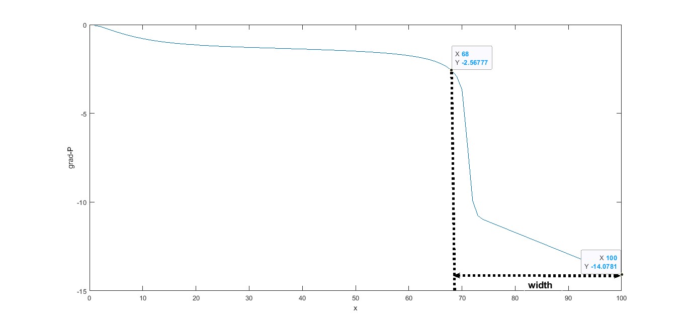
However for pic2 below it shouldn't as there is no steep gradient compared to pic1
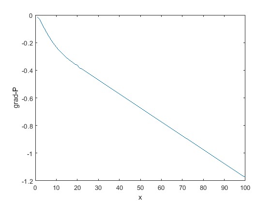
The code is as below:
clear width;
global width;
global data;
for i=1:max(length(data.variable.t))
for j=1:max(length(data.variable.x))-1
change_p = (abs(data.variable.gradpressure(i,j+1))-abs(data.variable.gradpressure(i,j)))/abs(data.variable.gradpressure(i,j));
%disp(change_p)
if change_p > 0.1
disp("steep gradient found")
width(j)=1-data.variable.x(j);
disp(width)
else
disp("no steep gradient found")
end
end
end
the data.variable.gradpressure is a 1000x100 matrix with t along the vertical and x along the horizontal.
with regards,
rc
Sub aspenaAdorption()
' Declare variables for the ACM application, document, and simulation
Dim ACMApp As Object
Dim ACMDocument As Object
Dim ACMSimulation As Object
' Create an instance of the ACM application
Set ACMApp = CreateObject("ACM Application")
' Use "ACM Application" for Aspen Custom Modeler
' Use "ADS Application" for Aspen Adsorption
' Make the ACM application visible
ACMApp.Visible = True
' Open the specified simulation document
Set ACMDocument = ACMApp.OpenDocument("C:\Users\user\Desktop\H2_Purification.acmf")
' Set the simulation object to the current simulation in the application
Set ACMSimulation = ACMApp.Simulation
' Set the simulation to run in dynamic mode
ACMSimulation.RunMode = "Dynamic"
' Run the simulation
ACMSimulation.Run (True)
' Check if the simulation was successful and display a message box
If ACMSimulation.Successful Then
MsgBox "Simulation Complete"
Else
MsgBox "Simulation Failed"
End If
' Quit the ACM application
ACMApp.Quit
End Sub
I have an old application that gives me an error when I run it. The error message states: "Could not find version 7.13 of the MCR. Attempting to load mclmcrrt713.dll. Please install the correct version of the MCR." I tried to install this version, but it is no longer available. Any help would be highly appreciated. Thanks!
In the program given below I fail to obtaine real pole as title in intger format if anyone know please guide me
num1=[1 -1];
den1=conv([1 1],conv([1 2+2j],[1 2-2j]));
G=tf(num1,den1);
P=pole(G);
Z = zero(G);
formatSpec='%s,%i,%f+%fi,%i';
a="Root Locus of ";
b='step response of';
figure(17)
rlocus(G)
p=sprintf(formatSpec,a,Z,P/1i,P(3,1));
title(p);
An option for 10th degree polynomials but no weighted linear least squares. Seriously? Jesse