eqn =
主要内容
搜索
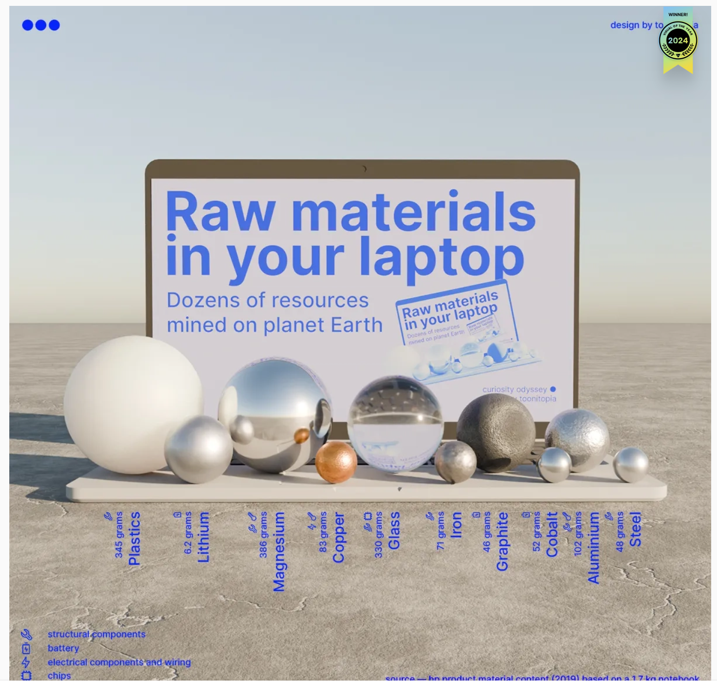
Check out this 3D chart that won Visual Of The Year for 2024 by Visual Capitalist. It's a mashup between a 3D bubblechart and a categorical bar plot yet the only graphical components are the x-axis labels and the legend. Not only does it show relative proportions of material in a laptop but it also shows what the raw material looks like.
I love the idea of analog data visualization. I wonder if any readers have made a analog "chart".
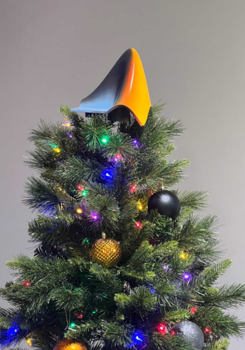
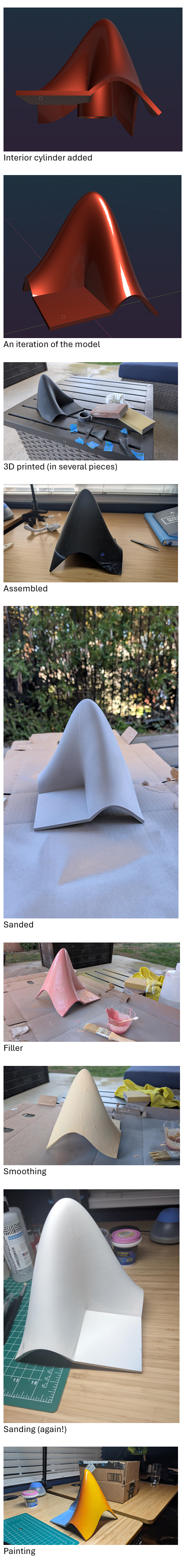
What better way to add a little holiday magic than the L-shaped membrane atop your evergreen? My colleagues output the shape and then added some thickness and an interior cylinder in Blender. Then, the shape was exported to STL and 3D printed (in several pieces). Then glued, sanded, primed, sanded again and painted. If you like, the STL file is attached. Thank you to https://blogs.mathworks.com/community/2013/06/20/paul-prints-the-l-shaped-membrane/ and a tip of the hat to MATLAB Ornament. Happy Holidays!
The MATLAB Online Training Suite has been updated in the areas of Deep Learning and traditional Machine Learning! These are great self-paced courses that can get you from zero to hero pretty quickly.
Deep Learning Onramp (Free to everyone!) has been updated to use the dlnetwork workflow, such as the trainnet function, which became the preferred method for creating and training deep networks in R2024a.
- Content streamlined to reduce the focus on data processing and feature extraction, and emphasize the machine learning workflow.
- Course example simplified by using a sample of the original data.
- Classification Learner used in the course where appropriate.
The rest of the updates are for subscribers to the full Online Training Suite
The Deep Learning Techniques in MATLAB for Image Applications learning path teaches skills to tackle a variety of image applications. It is made up of the following four short courses:
- Explore Convolutional Neural Networks
- Tune Deep Learning Training Options
- Regression with Deep Learning
- Object Detection with Deep Learning
Two more deep learning short courses are also available:
The Machine Learning Techniques in MATLAB learning path helps learners build their traditional machine learning skill set:
I'm beginning this MATLAB-based numerical methods class, and as I was thinking back to my previous MATLAB/Simulink classes, I definitely remember some projects more fondly than others. One of my most memorable was where I had to use MATLAB to analyze electrocardiogram (ECG) peaks. What about you guys? What are some of the best (or worst 🤭) MATLAB projects or assignments you've been given in the past?
Speaking as someone with 31+ years of experience developing and using imshow, I want to advocate for retiring and replacing it.
The function imshow has behaviors and defaults that were appropriate for the MATLAB and computer monitors of the 1990s, but which are not the best choice for most image display situations in today's MATLAB. Also, the 31 years have not been kind to the imshow code base. It is a glitchy, hard-to-maintain monster.
My new File Exchange function, imview, illustrates the kind of changes that I think should be made. The function imview is a much better MATLAB graphics citizen and produces higher quality image display by default, and it dispenses with the whole fraught business of trying to resize the containing figure. Although this is an initial release that does not yet support all the useful options that imshow does, it does enough that I am prepared to stop using imshow in my own work.
The Image Processing Toolbox team has just introduced in R2024b a new image viewer called imageshow, but that image viewer is created in a special-purpose window. It does not satisfy the need for an image display function that works well with the axes and figure objects of the traditional MATLAB graphics system.
I have published a blog post today that describes all this in more detail. I'd be interested to hear what other people think.
Note: Yes, I know there is an Image Processing Toolbox function called imview. That one is a stub for an old toolbox capability that was removed something like 15+ years ago. The only thing the toolbox imview function does now is call error. I have just submitted a support request to MathWorks to remove this old stub.
The int function in the Symbolic Toolbox has a hold/release functionality wherein the expression can be held to delay evaluation
syms x I
eqn = I == int(x,x,'Hold',true)
which allows one to show the integral, and then use release to show the result
release(eqn)
Maybe it would be nice to be able to hold/release any symbolic expression to delay the engine from doing evaluations/simplifications that it typically does. For example:
x*(x+1)/x, sin(sym(pi)/3)

If I'm trying to show a sequence of steps to develop a result, maybe I want to explicitly keep the x/x in the first case and then say "now the x in the numerator and denominator cancel and the result is ..." followed by the release command to get the final result.
Perhaps held expressions could even be nested to show a sequence of results upon subsequent releases.
Held expressions might be subject to other limitations, like maybe they can't be fplotted.
Seems like such a capability might not be useful for problem solving, but might be useful for exposition, instruction, etc.
Always and almost immediately!
26%
Never
30%
After validating existing code
15%
Y'all get the new releases?
29%
1843 个投票
Many of my best friends at MathWorks speak Spanish as their first language and we have a large community of Spanish-speaking users. You can see good evidence of this by checking out our relatively new Spanish YouTube channel which recently crossed the 10,000 subscriber mark
I've always used MATLAB with other languages. In the early days, C and C++ via mex files were the most common ways I spliced two languages together. Other than that I've also used MATLAB with Java, Excel and even Fortran.
In more recent years, Python is the language I tend to use most alongside MATLAB and support for this combination is steadily improving. In my latest blog post, I show how easy it has become to use Python's Numpy with MATLAB.
Have you used this functionality much? If so, what for? How well did it work for you?
I am inspired by the latest video from YouTube science content creator Veritasium on his distinct yet thorough explanation on how rainbows work. In his video, he set up a glass sphere experiment representing how light rays would travel inside a raindrop that ultimately forms the rainbow. I highly recommend checking it out.
In the meantime, I created an interactive MATLAB App in MATLAB Online using App Designer to visualize the light paths going through a spherical raindrop with numerical calculations along the way. While I've seen many diagrams out there showing the light paths, I haven't found any doing calculations in each step. Hence I created an app in MATLAB to show the calculations along with the visualizations as one varies the position of the incoming light ray.
Demo video:
For more information about the app and how to open it and play around with it in MATLAB Online, please check out my blog article:

Our MathWorks Usability Team is working on an accessibility project and they want to interview people who use MATLAB and also have experience with screen readers.
If you fit the criteria and are interested, sign up here https://www.mathworks.com/products/usability.html?tfa_30=A11Y
I wish I knew more about the intended evolution of the capabilities of the function arguments block. I love implementing function syntaxes using this relatively new form, but it doesn't yet handle some function syntax design patterns that I think are valuable and worth keeping.
For example, some functions take an input quantity that can something numeric, or it can be an option string that descriptively names a particular value of that quantity. One example is dateshift(t,"dayofweek",dow), where dow can be an integer from 1 to 7, or it can be one of the option strings "weekday" or "weekend".
Another example is Image Processing Toolbox that take a connectivity specifier as input. The function bwconncomp is one particular case. Connectivity can be specified using certain scalars, certain arrays, or the option string "maximal".
I think this is a worthwhile function design pattern, but I don't think the arguments block validation functionality supports it well (unless you use a lot of extra code that duplicates standard MATLAB behavior, which undermines the value of the arguments block).
MathWorkers - believe me, I know that it is not in your DNA to discuss future features. But would anyone care to offer a hint about directions for the arguments block functionality?

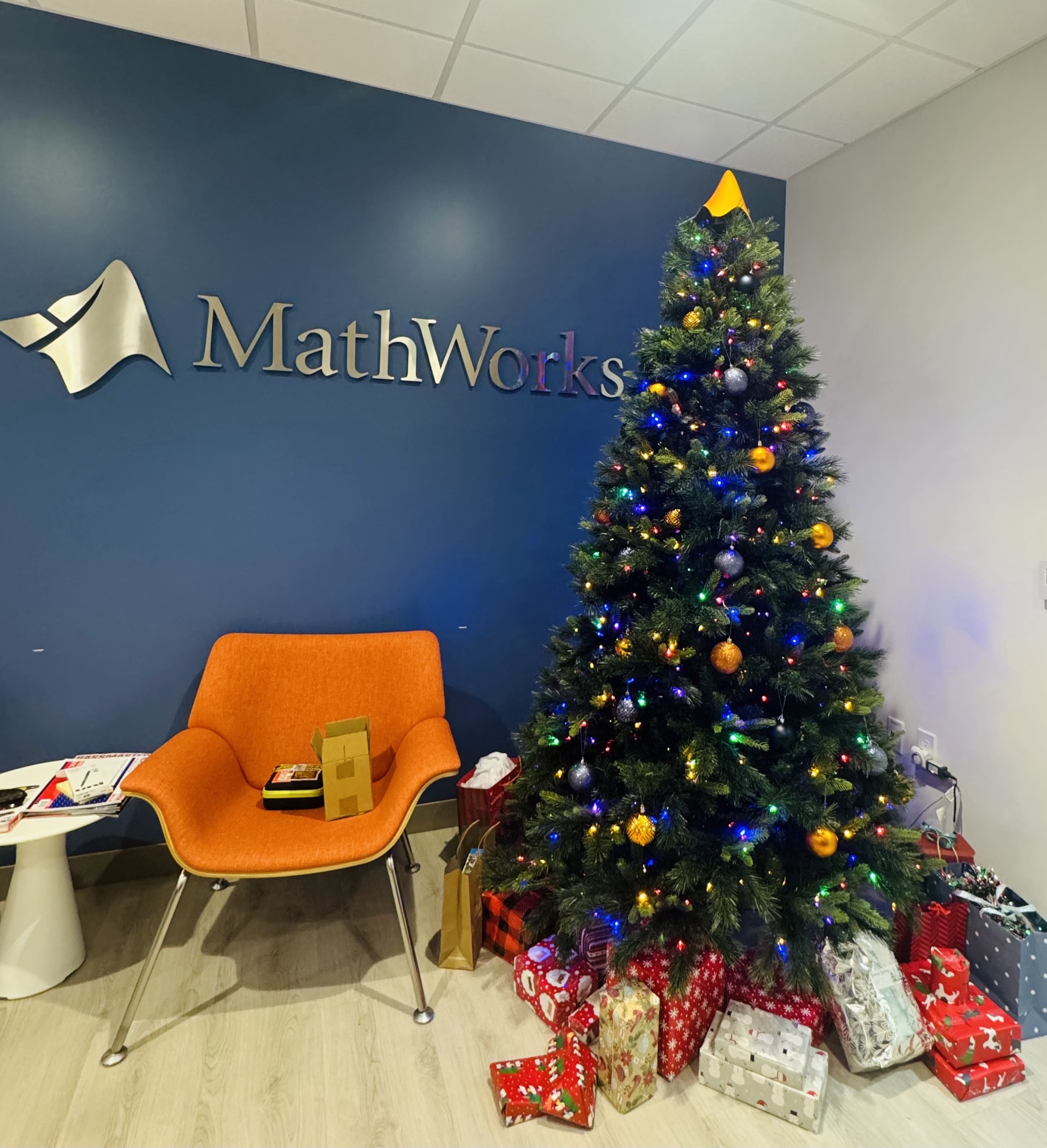
Christmas season is underway at my house:

(Sorry - the ornament is not available at the MathWorks Merch Shop -- I made it with a 3-D printer.)
At the present time, the following problems are known in MATLAB Answers itself:
- Symbolic output is not displaying. The work-around is to disp(char(EXPRESSION)) or pretty(EXPRESSION)
- Symbolic preferences are sometimes set to non-defaults
Just shared an amazing YouTube video that demonstrates a real-time PID position control system using MATLAB and Arduino.
I don't like the change
16%
I really don't like the change
29%
I'm okay with the change
24%
I love the change
11%
I'm indifferent
11%
I want both the web & help browser
11%
38 个投票
We are thrilled to announce the grand prize winners of our MATLAB Shorts Mini Hack contest! This year, we invited the MATLAB Graphics and Charting team, the authors of the MATLAB functions used in every entry, to be our judges. After careful consideration, they have selected the top three winners:
Judge comments: Realism & detailed comments; wowed us with Manta Ray
2nd place – Jenny Bosten
Judge comments: Topical hacks : Auroras & Wind turbine; beautiful landscapes & nightscapes
3rd place - Vasilis Bellos
Judge comments: Nice algorithms & extra comments; can’t go wrong with Pumpkins
Judge comments: Impressive spring & cubes!
In addition, after validating the votes, we are pleased to announce the top 10 participants on the leaderboard:
Congratulations to all! Your creativity and skills have inspired many of us to explore and learn new skills, and make this contest a big success!
您也可以从以下列表中选择网站:
美洲
- América Latina (Español)
- Canada (English)
- United States (English)
欧洲
- Belgium (English)
- Denmark (English)
- Deutschland (Deutsch)
- España (Español)
- Finland (English)
- France (Français)
- Ireland (English)
- Italia (Italiano)
- Luxembourg (English)
- Netherlands (English)
- Norway (English)
- Österreich (Deutsch)
- Portugal (English)
- Sweden (English)
- Switzerland
- United Kingdom(English)
亚太
- Australia (English)
- India (English)
- New Zealand (English)
- 中国
- 日本Japanese (日本語)
- 한국Korean (한국어)