Results for
- Tips & tricks: Discuss strategies for solving Cody problems that you've found effective.
- Ideas or suggestions for improvement: Have thoughts on how to make Cody better? We'd love to hear them.
- Issues: Encountering difficulties or bugs with Cody? Let us know so we can address them.
- Requests for guidance: Stuck on a Cody problem? Ask for advice or hints, but make sure to show your efforts in attempting to solve the problem first.
- General discussions: Anything else related to Cody that doesn't fit into the above categories.
- Comments on specific Cody problems: Examples include unclear problem descriptions or incorrect testing suites.
- Comments on specific Cody solutions: For example, you find a solution creative or helpful.
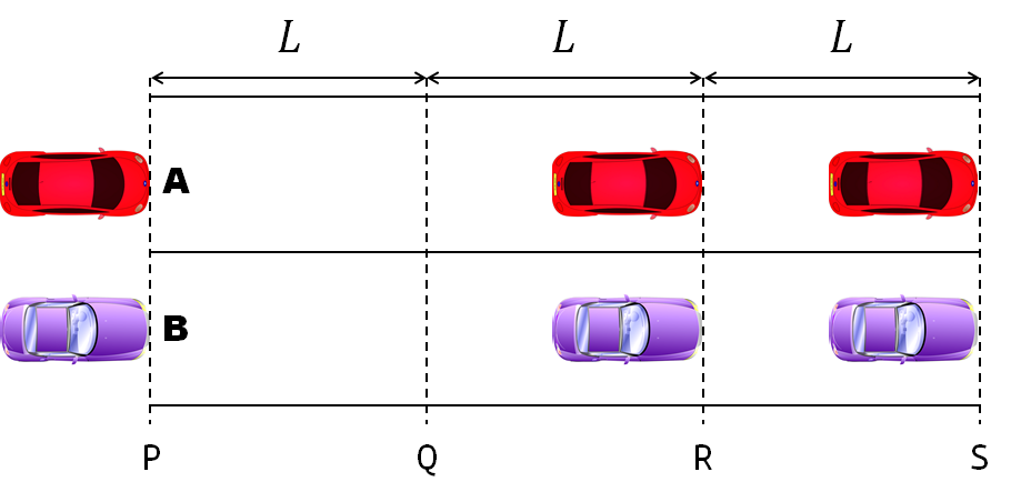
- Car A moves with constant velocity v.
- Car B starts to move when Car A passes through the point P.
- Car B undergoes...
- uniform acc. motion from P to Q.
- uniform velocity motion from Q to R.
- uniform acc. motion from R to S.
- Car A and B pass through the point R simultaneously.
- Car A and B arrive at the point S simultaneously.


Hello MathWorks Community,
I am excited to announce that I am currently working on a book project centered around Matrix Algebra, specifically designed for MATLAB users. This book aims to cater to undergraduate students in engineering, where Matrix Algebra serves as a foundational element.
Matrix Algebra is not only pivotal in understanding complex engineering concepts but also in applying these principles effectively in various technological solutions. MATLAB, renowned for its powerful computational capabilities, is an excellent tool to explore and implement these concepts, making it a perfect companion for this book.
As I embark on this journey to create a resource that bridges theoretical matrix algebra with practical MATLAB applications, I am looking for one or two knowledgeable individuals who have a firm grasp of both subjects. If you have experience in teaching or applying matrix algebra in engineering contexts and are familiar with MATLAB, your contribution could be invaluable.
Collaborators will help in shaping the content to ensure it is educational, engaging, and technically robust, making complex concepts accessible and applicable for students.
If you are interested in contributing to this project or know someone who might be, please reach out to discuss how we can work together to make this book a valuable resource for engineering students.
Thank you and looking forward to your participation!

- https://www.mathworks.com/matlabcentral/answers/480389-colored-line-plot-according-to-a-third-variable
- https://www.mathworks.com/matlabcentral/answers/2092641-how-to-solve-a-problem-with-the-generation-of-multiple-colored-segments-on-one-line-in-matlab-plot
- https://www.mathworks.com/matlabcentral/answers/5042-how-do-i-vary-color-along-a-2d-line
- https://www.mathworks.com/matlabcentral/answers/1917650-how-to-plot-a-trajectory-with-varying-colour
- https://www.mathworks.com/matlabcentral/answers/1917650-how-to-plot-a-trajectory-with-varying-colour
- https://www.mathworks.com/matlabcentral/answers/511523-how-to-create-plot3-varying-color-figure
- https://www.mathworks.com/matlabcentral/answers/393810-multiple-colours-in-a-trajectory-plot
- https://www.mathworks.com/matlabcentral/answers/523135-creating-a-rainbow-colour-plot-trajectory
- https://www.mathworks.com/matlabcentral/answers/469929-how-to-vary-the-color-of-a-dynamic-line
- https://www.mathworks.com/matlabcentral/answers/585011-how-could-i-adjust-the-color-of-multiple-lines-within-a-graph-without-using-the-default-matlab-colo
- https://www.mathworks.com/matlabcentral/answers/517177-how-to-interpolate-color-along-a-curve-with-specific-colors
- https://www.mathworks.com/matlabcentral/answers/281645-variate-color-depending-on-the-y-value-in-plot
- https://www.mathworks.com/matlabcentral/answers/439176-how-do-i-vary-the-color-along-a-line-in-polar-coordinates
- https://www.mathworks.com/matlabcentral/answers/1849193-creating-rainbow-coloured-plots-in-3d
- https://groups.google.com/g/comp.soft-sys.matlab/c/cLgjSeEC15I?hl=en&pli=1 (a question asked in 1999!)
- ... the list goes on, and on, and on...
- https://undocumentedmatlab.com/articles/plot-line-transparency-and-color-gradient
- https://www.mathworks.com/matlabcentral/fileexchange/19476-colored-line-or-scatter-plot
- https://www.mathworks.com/matlabcentral/fileexchange/23566-3d-colored-line-plot
- https://www.mathworks.com/matlabcentral/fileexchange/30423-conditionally-colored-line-plot
- https://www.mathworks.com/matlabcentral/fileexchange/14677-cline
- https://www.mathworks.com/matlabcentral/fileexchange/8597-plot-3d-color-line
- https://www.mathworks.com/matlabcentral/fileexchange/39972-colormapline-color-changing-2d-or-3d-line
- https://www.mathworks.com/matlabcentral/fileexchange/37725-conditionally-colored-plot-ccplot
- https://www.mathworks.com/matlabcentral/fileexchange/11611-linear-2d-plot-with-rainbow-color
- https://www.mathworks.com/matlabcentral/fileexchange/26692-color_line
- https://www.mathworks.com/matlabcentral/fileexchange/32911-plot3rgb
- And perhaps more?
- https://www.mathworks.com/videos/coloring-a-line-based-on-height-gradient-or-some-other-value-in-matlab-97128.html
- https://www.mathworks.com/videos/making-a-multi-color-line-in-matlab-97127.html
- https://www.mathworks.com/matlabcentral/fileexchange/95663-color-trajectory-plot (contributed by a MathWorks staff member)
- And perhaps more?
- 행렬의 두 row 벡터로 정의되는 평행사변형의 면적입니다.
- 물론 두 column 벡터로 정의되는 평행사변형의 면적이기도 합니다.
- 좀 더 정확히는 signed area입니다. 면적이 음수가 될 수도 있다는 뜻이죠.
- 행렬의 두 행(또는 두 열)을 맞바꾸면 행렬식의 부호도 바뀌고 면적의 부호도 바뀌어야합니다.
- 각 row 벡터(또는 각 column 벡터)로 정의되는 N차원 공간의 평행면체(?)의 signed area입니다.
- 제대로 이해하려면 대수학의 개념을 많이 가지고 와야 하는데 자세한 설명은 생략합니다.(=저도 모른다는 뜻)
- 더 자세히 알고 싶으시면 수학하는 만화의 '넓이 이야기' 편을 추천합니다.
- 수학적인 정의를 알고 싶으시면 위키피디아를 보시면 됩니다.
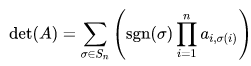
- 이렇게 생겼습니다. 좀 무섭습니다.
- 2 x 2 행렬에 대해서 이것을 수식 없이 그림만으로 증명하는 과정입니다.
- gif 생성에는 ScreenToGif를 사용했습니다. (gif 만들기엔 이게 킹왕짱인듯)
- An area of a parallelogram defined by two row vectors.
- Of course, same one defined by two column vectors.
- Precisely, a signed area, which means area can be negative.
- If two rows (or columns) are swapped, both the sign of determinant and area change.
- Signed area of parallelepiped defined by rows (or columns) of the matrix in n-dim space.
- For a full understanding, a lot of concepts from abstract algebra should be brought, which I will not write here. (Cuz I don't know them.)
- For a mathematical definition of determinant, visit wikipedia.

- A little scary, isn't it?
- A process to prove the equality of the determinant of 2 x 2 matrix and the area of parallelogram.
- ScreenToGif is used to generate gif animation (which is, to me, the easiest way to make gif).


您也可以从以下列表中选择网站:
美洲
- América Latina (Español)
- Canada (English)
- United States (English)
欧洲
- Belgium (English)
- Denmark (English)
- Deutschland (Deutsch)
- España (Español)
- Finland (English)
- France (Français)
- Ireland (English)
- Italia (Italiano)
- Luxembourg (English)
- Netherlands (English)
- Norway (English)
- Österreich (Deutsch)
- Portugal (English)
- Sweden (English)
- Switzerland
- United Kingdom(English)
亚太
- Australia (English)
- India (English)
- New Zealand (English)
- 中国
- 日本Japanese (日本語)
- 한국Korean (한국어)