搜索
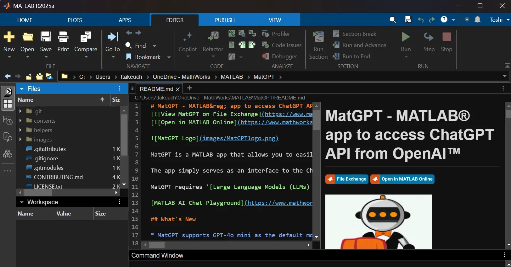
In case you missed it in my overview of the MATLAB R2025a release, Markdown support has been greatly improved. This picture says it all
Untapped Potential for Output-arguments Block
MATLAB has a very powerful feature in its arguments blocks. For example, the following code for a function (or method):
- clearly outlines all the possible inputs
- provides default values for each input
- will produce auto-complete suggestions while typing in the Editor (and Command Window in newer versions)
- checks each input against validation functions to enforce size, shape (e.g., column vs. row vector), type, and other options (e.g., being a member of a set)
function [out] = sample_fcn(in)
arguments(Input)
in.x (:, 1) = []
in.model_type (1, 1) string {mustBeMember(in.model_type, ...
["2-factor", "3-factor", "4-factor"])} = "2-factor"
in.number_of_terms (1, 1) {mustBeMember(in.number_of_terms, 1:5)} = 1
in.normalize_fit (1, 1) logical = false
end
% function logic ...
end
If you do not already use the arguments block for function (or method) inputs, I strongly suggest that you try it out.
The point of this post, though, is to suggest improvements for the output-arguments block, as it is not nearly as powerful as its input-arguments counterpart. I have included two function examples: the first can work in MATLAB while the second does not, as it includes suggestions for improvements. Commentary specific to each function is provided completely before the code. While this does necessitate navigating back and forth between functions and text, this provides for an easy comparison between the two functions which is my main goal.
Current Implementation
The input-arguments block for sample_fcn begins the function and has already been discussed. A simple output-arguments block is also included. I like to use a single output so that additional fields may be added at a later point. Using this approach simplifies future development, as the function signature, wherever it may be used, does not need to be changed. I can simply add another output field within the function and refer to that additional field wherever the function output is used.
Before beginning any logic, sample_fcn first assigns default values to four fields of out. This is a simple and concise way to ensure that the function will not error when returning early.
The function then performs two checks. The first is for an empty input (x) vector. If that is the case, nothing needs to be done, as the function simply returns early with the default output values that happen to apply to the inability to fit any data.
The second check is for edge cases for which input combinations do not work. In this case, the status is updated, but default values for all other output fields (which are already assigned) still apply, so no additional code is needed.
Then, the function performs the fit based on the specified model_type. Note that an otherwise case is not needed here, since the argument validation for model_type would not allow any other value.
At this point, the total_error is calculated and a check is then made to determine if it is valid. If not, the function again returns early with another specific status value.
Finally, the R^2 value is calculated and a fourth check is performed. If this one fails, another status value is assigned with an early return.
If the function has passed all the checks, then a set of assertions ensure that each of the output fields are valid. In this case, there are eight specific checks, two for each field.
If all of the assertions also pass, then the final (successful) status is assigned and the function returns normally.
function [out] = sample_fcn(in)
arguments(Input)
in.x (:, 1) = []
in.model_type (1, 1) string {mustBeMember(in.model_type, ...
["2-factor", "3-factor", "4-factor"])} = "2-factor"
in.number_of_terms (1, 1) {mustBeMember(in.number_of_terms, 1:5)} = 1
in.normalize_fit (1, 1) logical = false
end
arguments(Output)
out struct
end
%%
out.fit = [];
out.total_error = [];
out.R_squared = NaN;
out.status = "Fit not possible for supplied inputs.";
%%
if isempty(in.x)
return
end
%%
if ((in.model_type == "2-factor") && (in.number_of_terms == 5)) || ... % other possible logic
out.status = "Specified combination of model_type and number_of_terms is not supported.";
return
end
%%
switch in.model_type
case "2-factor"
out.fit = % code for 2-factor fit
case "3-factor"
out.fit = % code for 3-factor fit
case "4-factor"
out.fit = % code for 4-factor fit
end
%%
out.total_error = % calculation of error
if ~isfinite(out.total_error)
out.status = "The total_error could not be calculated.";
return
end
%%
out.R_squared = % calculation of R^2
if out.R_squared > 1
out.status = "The R^2 value is out of bounds.";
return
end
%%
assert(iscolumn(out.fit), "The fit vector is not a column vector.");
assert(size(out.fit) == size(in.x), "The fit vector is not the same size as the input x vector.");
assert(isscalar(out.total_error), "The total_error is not a scalar.");
assert(isfinite(out.total_error), "The total_error is not finite.");
assert(isscalar(out.R_squared), "The R^2 value is not a scalar.");
assert(isfinite(out.R_squared), "The R^2 value is not finite.");
assert(isscalar(out.status), "The status is not a scalar.");
assert(isstring(out.status), "The status is not a string.");
%%
out.status = "The fit was successful.";
end
Potential Implementation
The second function, sample_fcn_output_arguments, provides essentially the same functionality in about half the lines of code. It is also much clearer with respect to the output. As a reminder, this function structure does not currently work in MATLAB, but hopefully it will in the not-too-distant future.
This function uses the same input-arguments block, which is then followed by a comparable output-arguments block. The first unsupported feature here is the use of name-value pairs for outputs. I would much prefer to make these assignments here rather than immediately after the block as in the sample_fcn above, which necessitates four more lines of code.
The mustBeSameSize validation function that I use for fit does not exist, but I really think it should; I would use it a lot. In this case, it provides a very succinct way of ensuring that the function logic did not alter the size of the fit vector from what is expected.
The mustBeFinite validation function for out.total_error does not work here simply because of the limitation on name-value pairs; it does work for regular outputs.
Finally, the assignment of default values to output arguments is not supported.
The next three sections of sample_fcn_output_arguments match those of sample_fcn: check if x is empty, check input combinations, and perform fit logic. Following that, though, the functions diverge heavily, as you might expect. The two checks for total_error and R^2 are not necessary, as those are covered by the output-arguments block. While there is a slight difference, in that the specific status values I assigned in sample_fcn are not possible, I would much prefer to localize all these checks in the arguments block, as is already done for input arguments.
Furthermore, the entire section of eight assertions in sample_fcn is removed, as, again, that would be covered by the output-arguments block.
This function ends with the same status assignment. Again, this is not exactly the same as in sample_fcn, since any failed assertion would prevent that assignment. However, that would also halt execution, so it is a moot point.
function [out] = sample_fcn_output_arguments(in)
arguments(Input)
in.x (:, 1) = []
in.model_type (1, 1) string {mustBeMember(in.model_type, ...
["2-factor", "3-factor", "4-factor"])} = "2-factor"
in.number_of_terms (1, 1) {mustBeMember(in.number_of_terms, 1:5)} = 1
in.normalize_fit (1, 1) logical = false
end
arguments(Output)
out.fit (:, 1) {mustBeSameSize(out.fit, in.x)} = []
out.total_error (1, 1) {mustBeFinite(out.total_error)} = []
out.R_squared (1, 1) {mustBeLessThanOrEqual(out.R_squared, 1)} = NaN
out.status (1, 1) string = "Fit not possible for supplied inputs."
end
%%
if isempty(in.x)
return
end
%%
if ((in.model_type == "2-factor") && (in.number_of_terms == 5)) || ... % other possible logic
out.status = "Specified combination of model_type and number_of_terms is not supported.";
return
end
%%
switch in.model_type
case "2-factor"
out.fit = % code for 2-factor fit
case "3-factor"
out.fit = % code for 3-factor fit
case "4-factor"
out.fit = % code for 4-factor fit
end
%%
out.status = "The fit was successful.";
end
Final Thoughts
There is a significant amount of unrealized potential for the output-arguments block. Hopefully what I have provided is helpful for continued developments in this area.
What are your thoughts? How would you improve arguments blocks for outputs (or inputs)? If you do not already use them, I hope that you start to now.
キーと値の組み合わせでデータを格納できるディクショナリ。R2022bでdictionaryコマンドが登場し、最近のバージョンではreaddictionaryとwritedictionaryでJSONファイルからの読み込み・書き込みにも対応しました。
私はMIDIデータからピアノの演奏動画を作るプログラムで、ディクショナリを使いました。音のノート番号をキーにして、patchで白と黒で鍵盤を塗りつぶしたmatlab.graphics.Graphicsデータ型を値にしたディクショナリで保存して、MIDIで鳴らされた音のノート番号からlookupでグラフのオブジェクトを取得し、FaceColorを変更してハイライトするというもの。

皆さんはディクショナリを使ってますか? もし使っていたら、どういう活用をしているか、聞かせてください!
どの方法を使う事が多いですか?他によく使う方法があれば教えてくださいー。
方法①
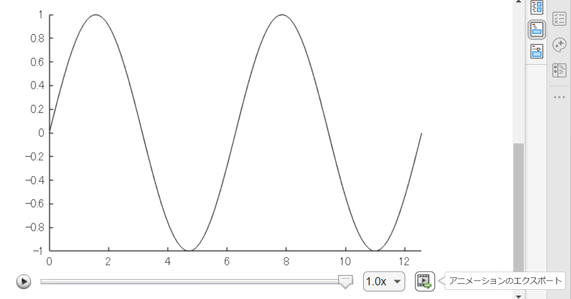
Livescript 上で for ループ内で描画を編集させて描いた動画は「アニメーションのエクスポート」から動画ファイルに出力するのが一番簡単ですね。再生速度やら細かい設定ができない点は要注意。
方法②
exportgraphics 関数で "Append" オプション指定で実現できるようになった(R2022a から)のでこれも便利ですね。
N = 100;
x = linspace(0,4*pi,N);
y = sin(x);
filename = 'animation_sample.gif'; % Specify the output file name
if exist(filename,'file')
delete(filename)
end
h = animatedline;
axis([0,4*pi,-1,1]) % x軸の表示範囲を固定
for k = 1:length(x)
addpoints(h,x(k),y(k)); % ループでデータを追加
exportgraphics(gca,filename,"Append",true)
end
方法③
R2021b 以前のバージョンだとこんな感じ。
各ループで画面キャプチャして、imwrite で動画ファイルにフレーム追加していくイメージです。"DelayTime" を使って細かい指定ができるので、必要に応じて今でも利用します。
for k = 1:length(x)
addpoints(h,x(k),y(k)); % ループでデータを追加
drawnow % グラフアップデート
frame = getframe(gcf); % Figure 画面をムービーフレーム(構造体)としてキャプチャ
tmp = frame2im(frame); % 画像に変更
[A,map] = rgb2ind(tmp,256); % RGB -> インデックス画像に
if k == 1 % 新規 gif ファイル作成
imwrite(A,map,filename,'gif','LoopCount',Inf,'DelayTime',0.2);
else % 以降、画像をアペンド
imwrite(A,map,filename,'gif','WriteMode','append','DelayTime',0.2);
end
end
I saw this on Reddit and thought of the past mini-hack contests. We have a few folks here who can do something similar with MATLAB.
これからは生成AIでコードを1から書くという事が減ってくるのかと思いますが,皆さんがMATLABのコードを書く時に意識しているご自身のルールのようなものがあれば教えてください.
MATLAB言語は柔軟に書けますが,自然と個人個人のルールというものが出来上がってきているのでは,と思います.
私はParameter, Valueペアの引数がある関数はそれぞれのペアを新しい行に書く,というのをよくやります.
h = plot(x, y, "ro-", ...
"LineWidth", 2, ...
"MarkerSize", 10, ...
"MarkerFaceColor", "g");
Parameter=Valueでも同じです.
h = plot(x, y, "ro-", ...
LineWidth = 2, ...
MarkerSize = 10, ...
MarkerFaceColor = "g");
また,一時期は "=" を揃えることもやってました(今はやってませんが).
h = plot(x, y, "ro-", ...
LineWidth = 2, ...
MarkerSize = 10, ...
MarkerFaceColor = "g");
皆さんにはどのようなルールがありますか?
The Graphics and App Building Blog just launched its first article on R2025a features, authored by Chris Portal, the director of engineering for the MATLAB graphics and app building teams.
Over the next few months, we'll publish a series of articles that showcase our updated graphics system, introduce new tools and features, and provide valuable references enriched by the perspectives of those involved in their development.
To stay updated, you can subscribe to the blog (look for the option in the upper left corner of the blog page). We also encourage you to join the conversation—your comments and questions under each article help shape the discussion and guide future content.

I had an error in the web version Matlab, so I exited and came back in, and this boy was plotted.
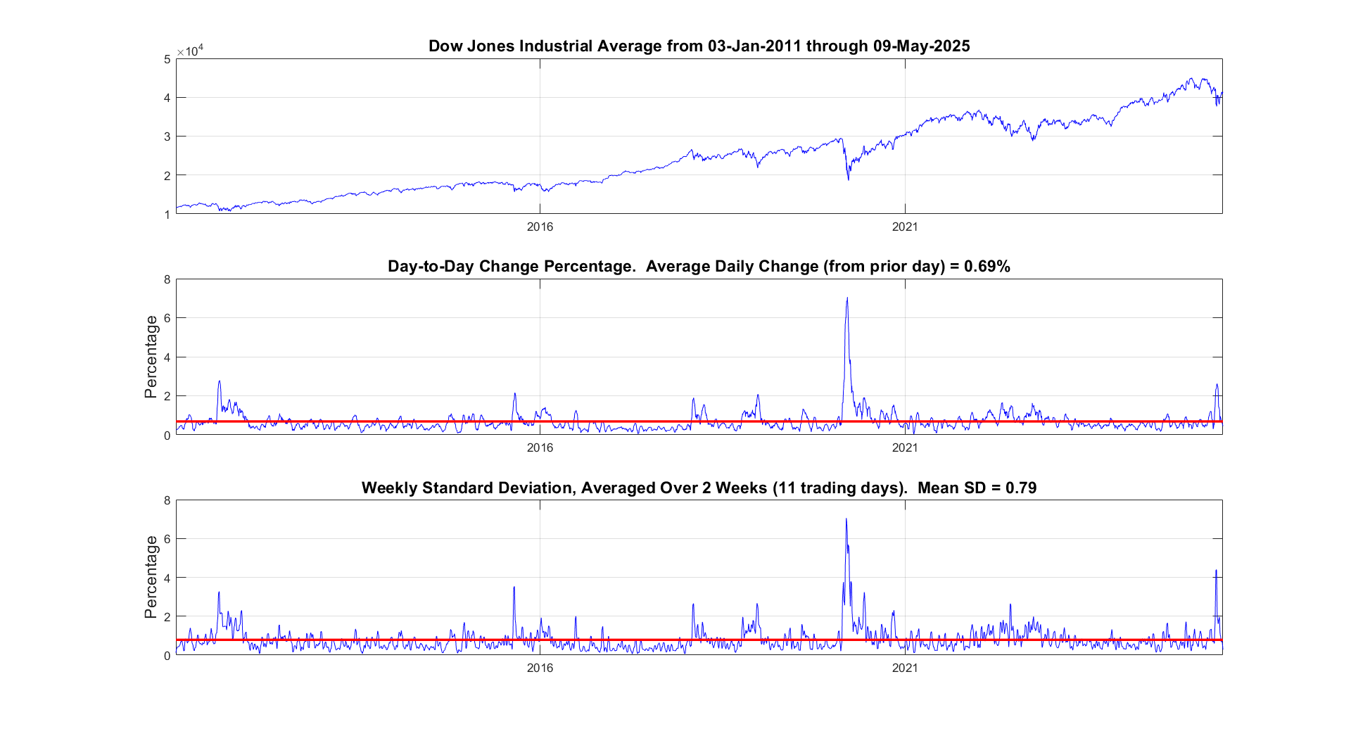
It seems like the financial news is always saying the stock market is especially volatile now. But is it really? This code will show you the daily variation from the prior day. You can see that the average daily change from one day to the next is 0.69%. So any change in the stock market from the prior day less than about 0.7% or 1% is just normal "noise"/typical variation. You can modify the code to adjust the starting date for the analysis. Data file (Excel workbook) is attached (hopefully - I attached it twice but it's not showing up yet).
% Program to plot the Dow Jones Industrial Average from 1928 to May 2025, and compute the standard deviation.
% Data available for download at https://finance.yahoo.com/quote/%5EDJI/history?p=%5EDJI
% Just set the Time Period, then find and click the download link, but you ned a paid version of Yahoo.
%
% If you have a subscription for Microsoft Office 365, you can also get historical stock prices.
% Reference: https://support.microsoft.com/en-us/office/stockhistory-function-1ac8b5b3-5f62-4d94-8ab8-7504ec7239a8#:~:text=The%20STOCKHISTORY%20function%20retrieves%20historical,Microsoft%20365%20Business%20Premium%20subscription.
% For example put this in an Excel Cell
% =STOCKHISTORY("^DJI", "1/1/2000", "5/10/2025", 0, 1, 0, 1,2,3,4, 5)
% and it will fill out a table in Excel
%====================================================================================================================
clc; % Clear the command window.
close all; % Close all figures (except those of imtool.)
imtool close all; % Close all imtool figures if you have the Image Processing Toolbox.
clear; % Erase all existing variables. Or clearvars if you want.
workspace; % Make sure the workspace panel is showing.
format long g;
format compact;
fontSize = 14;
filename = 'Dow Jones Industrial Index.xlsx';
data = readtable(filename);
% Date,Close,Open,High,Low,Volume
dates = data.Date;
closing = data.Close;
volume = data.Volume;
% Define start date and stop date
startDate = datetime(2011,1,1)
stopDate = dates(end)
selectedDates = dates > startDate;
% Extract those dates:
dates = dates(selectedDates);
closing = closing(selectedDates);
volume = volume(selectedDates);
% Plot Volume
hFigVolume = figure('Name', 'Daily Volume');
plot(dates, volume, 'b-');
grid on;
xticks(startDate:calendarDuration(5,0,0):stopDate)
title('Dow Jones Industrial Average Volume', 'FontSize', fontSize);
hFig = figure('Name', 'Daily Standard Deviation');
subplot(3, 1, 1);
plot(dates, closing, 'b-');
xticks(startDate:calendarDuration(5,0,0):stopDate)
drawnow;
grid on;
caption = sprintf('Dow Jones Industrial Average from %s through %s', dates(1), dates(end));
title(caption, 'FontSize', fontSize);
% Get the average change from one trading day to the next.
diffs = 100 * abs(closing(2:end) - closing(1:end-1)) ./ closing(1:end-1);
subplot(3, 1, 2);
averageDailyChange = mean(diffs)
% Looks pretty noisy so let's smooth it for a nicer display.
numWeeks = 4;
diffs = sgolayfilt(diffs, 2, 5*numWeeks+1);
plot(dates(2:end), diffs, 'b-');
grid on;
xticks(startDate:calendarDuration(5,0,0):stopDate)
hold on;
line(xlim, [averageDailyChange, averageDailyChange], 'Color', 'r', 'LineWidth', 2);
ylabel('Percentage', 'FontSize', fontSize);
caption = sprintf('Day-to-Day Change Percentage. Average Daily Change (from prior day) = %.2f%%', averageDailyChange);
title(caption, 'FontSize', fontSize);
drawnow;
% Get the stddev over a 5 trading day window.
sd = stdfilt(closing, ones(5, 1));
% Get it relative to the magnitude.
sd = sd ./ closing * 100;
averageVariation = mean(sd)
numWeeks = 2;
% Looks pretty noisy so let's smooth it for a nicer display.
sd = sgolayfilt(sd, 2, 5*numWeeks+1);
% Plot it.
subplot(3, 1, 3);
plot(dates, sd, 'b-');
grid on;
xticks(startDate:calendarDuration(5,0,0):stopDate)
hold on;
line(xlim, [averageVariation, averageVariation], 'Color', 'r', 'LineWidth', 2);
ylabel('Percentage', 'FontSize', fontSize);
caption = sprintf('Weekly Standard Deviation, Averaged Over %d Weeks (%d trading days). Mean SD = %.2f', ...
numWeeks, 5*numWeeks+1, averageVariation);
title(caption, 'FontSize', fontSize);
% Maximize figure window.
g = gcf;
g.WindowState = 'maximized';
The following lines were added to the subplot function in version 2025a (line 291):
if ancestorFigure.Units == "normalized"
waitfor(ancestorFigure,'FigureViewReady',true);
end
That code isn't in version 2024a.
Because of this, I'm experiencing issues that cause the code to stop running when using subplot in this way:
figure('Units','normalized','Position',[0 0 0.3 0.3])
subplot(1,2,1)
...
Has anyone else encountered this error?
Does anyone understand the need for those lines of code?
As far as I can tell, there is still no official support for creating publication-ready tables from regression output, either as latex or natively. Although MATLAB isn't primarily statistical software, this still seems like an oversight, as almost any similar software has this capability built-in or as a package.
w = logspace(-1,3,100);
[m,p] = bode(tf(1,[1 1]),w);
size(m)
and therefore plotting requires an explicit squeeze (or rehape, or colon)
% semilogx(w,squeeze(db(m)))
Similarly, I'm using page* functions more regularly and am now generating 3D results whereas my old code would generate 2D. For example
x = [1;1];
theta = reshape(0:.1:2*pi,1,1,[]);
Z = [cos(theta), sin(theta);-sin(theta),cos(theta)];
y = pagemtimes(Z,x);
Now, plotting requires squeezing the inputs
% plot(squeeze(theta),squeeze(y))
Would there be any drawbacks to having plot, et. al., automagically apply squeeze to its inputs?
昨日 5/29 にお台場で MATLAB EXPO が開催されました。ご参加くださった方々ありがとうございました!
私は AI 関連のデモ展示で解説員としても立っておりましたが、立ち寄ってくださる方が絶えず、ずっと喋り続けてました。また、講演後に「さっきのすごくね?」という会話が漏れ聞こえてきたのがハイライト。
参加されたみなさま、印象に残ったこと・気になった講演・ポスター・デモ・新機能等あったら教えてください!(次回に向けて運営面での感想も)

The ability to plot multiple signals on a plot and then use the plot browser to interactively control which ones are displayed has been one of the most useful features of the plotting tools and many of my scripts embed the command to open it after results analysis and plotting. It's been removed in 2025A with the comment that the Property Inspector provides the alternative. It doesn't. Having to go back into the menu to select the plot edit features to get to the Property Inspector (which doesn't provide an efficient alternative to the plot browser) has made the workflow very inefficient. Please bring it back a.s.a.p. !!!!
以前のEXPOでも参加・聴講したことがある
67%
知り合いから聞いた
0%
MathWorksからのプロモーション,EXPOサイトで知った
0%
今年のEXPO会場でたまたま見かけた
0%
ライトニングトークって何?
33%
3 个投票
Due to MATLAB being banned in some mainland Chinese universities in 2020, in recent years a Chinese company called "Suzhou Tongyuan SoftControl" has completely imitated MATLAB’s behavior. Below are some screenshots as evidence. What is your opinion on this issue?

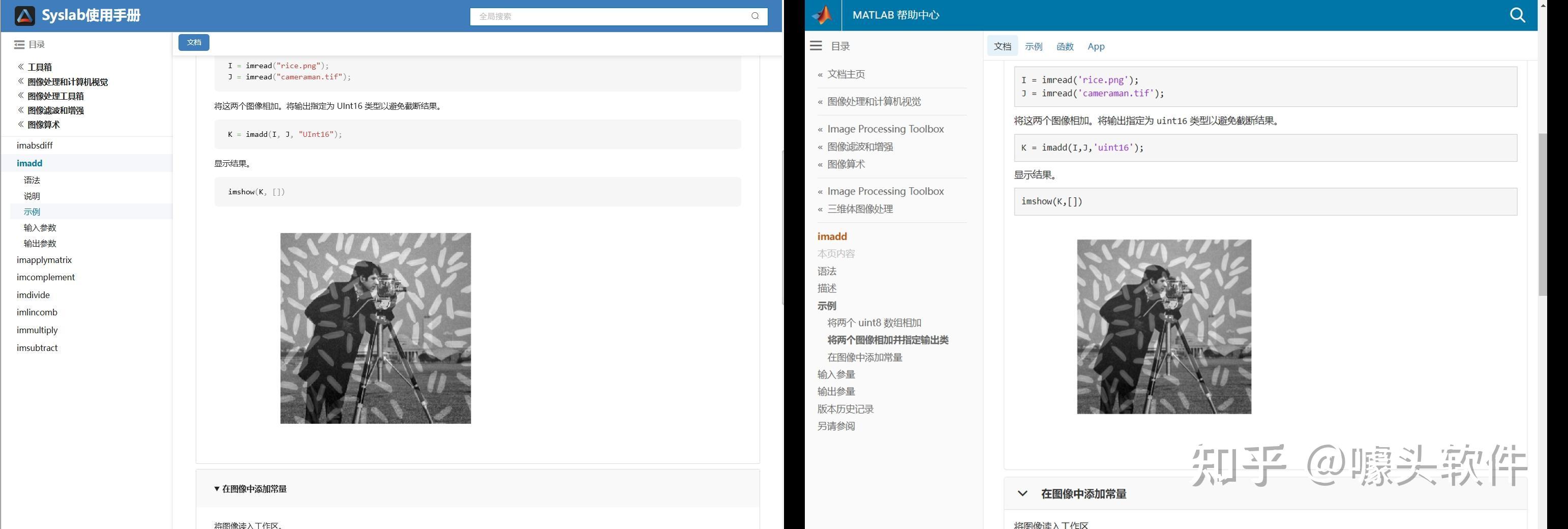

Source: Syslab 帮助文档-苏州同元软控
After waiting for a long time, the MathWorks official Community has finally resumed some of its functionalitys! Congratulations! Next, I’d like to share some thoughts to help prevent such outages from happening again, as they have affected far too many people.
- Almost all resources rely solely on MathWorks servers. Once a failure (or a ransomware attack) occurs, everything is paralyzed, and there isn’t even a temporary backup server? For a big company like MathWorks to have no contingency plan at all is eye-opening. This tells us that we should have our own temporary emergency servers!
- The impact should be minimized. For example, many users need to connect to the official servers to download various support packages, such as the “Deep Learning Toolbox Converter for ONNX Model Format.” Could these be backed up and mirrored to the “releases” section of a GitHub repository, so users in need can download them.
- A large proportion of users who have already installed MATLAB cannot access the online help documentation. Since R2023a, installing the help documentation locally has become optional. This only increases the burden on the servers? Moreover, the official website only hosts documentation for the past five years. That means after 2028, if I haven’t installed the local offline documentation, I won’t be able to access the online documentation for R2023a anymore?
Anything else you’d like to add? Feel free to leave a comment.
Any status updates on the license center and add on tool boxes?