ans = 
主要内容
Results for
As far as I know, starting from MATLAB R2024b, the documentation is defaulted to be accessed online. However, the problem is that every time I open the official online documentation through my browser, it defaults or forcibly redirects to the documentation hosted site for my current geographic location, often with multiple pop-up reminders, which is very annoying!

Suggestion: Could there be an option to set preferences linked to my personal account so that the documentation defaults to my chosen language preference without having to deal with “forced reminders” or “forced redirection” based on my geographic location? I prefer reading the English documentation, but the website automatically redirects me to the Chinese documentation due to my geolocation, which is quite frustrating!
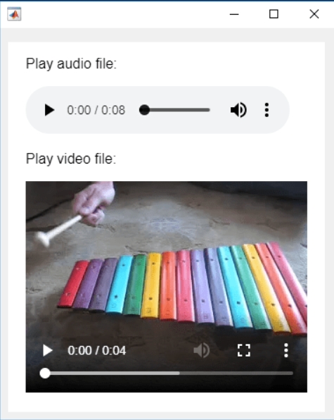
In the past two years, MATHWORKS has updated the image viewer and audio viewer, giving them a more modern interface with features like play, pause, fast forward, and some interactive tools that are more commonly found in typical third-party players. However, the video player has not seen any updates. For instance, the Video Viewer or vision.VideoPlayer could benefit from a more modern player interface. Perhaps I haven't found a suitable built-in player yet. It would be great if there were support for custom image processing and audio processing algorithms that could be played in a more modern interface in real time.
Additionally, I found it quite challenging to develop a modern video player from scratch in App Designer.(If there's a video component for that that would be great)
-----------------------------------------------------------------------------------------------------------------
BTW,the following picture shows the built-in function uihtml function showing a more modern playback interface with controls for play, pause and so on. But can not add real-time image processing algorithms within it.
Has this been eliminated? I've been at 31 or 32 for 30 days for awhile, but no badge. 10 badge was automatic.
Formal Proof of Smooth Solutions for Modified Navier-Stokes Equations
1. Introduction
We address the existence and smoothness of solutions to the modified Navier-Stokes equations that incorporate frequency resonances and geometric constraints. Our goal is to prove that these modifications prevent singularities, leading to smooth solutions.
2. Mathematical Formulation
2.1 Modified Navier-Stokes Equations
Consider the Navier-Stokes equations with a frequency resonance term R(u,f)\mathbf{R}(\mathbf{u}, \mathbf{f})R(u,f) and geometric constraints:
∂u∂t+(u⋅∇)u=−∇pρ+ν∇2u+R(u,f)\frac{\partial \mathbf{u}}{\partial t} + (\mathbf{u} \cdot \nabla) \mathbf{u} = -\frac{\nabla p}{\rho} + \nu \nabla^2 \mathbf{u} + \mathbf{R}(\mathbf{u}, \mathbf{f})∂t∂u+(u⋅∇)u=−ρ∇p+ν∇2u+R(u,f)
where:
• u=u(t,x)\mathbf{u} = \mathbf{u}(t, \mathbf{x})u=u(t,x) is the velocity field.
• p=p(t,x)p = p(t, \mathbf{x})p=p(t,x) is the pressure field.
• ν\nuν is the kinematic viscosity.
• R(u,f)\mathbf{R}(\mathbf{u}, \mathbf{f})R(u,f) represents the frequency resonance effects.
• f\mathbf{f}f denotes external forces.
2.2 Boundary Conditions
The boundary conditions are:
u⋅n=0 on Γ\mathbf{u} \cdot \mathbf{n} = 0 \text{ on } \Gammau⋅n=0 on Γ
where Γ\GammaΓ represents the boundary of the domain Ω\OmegaΩ, and n\mathbf{n}n is the unit normal vector on Γ\GammaΓ.
3. Existence and Smoothness of Solutions
3.1 Initial Conditions
Assume initial conditions are smooth:
u(0)∈C∞(Ω)\mathbf{u}(0) \in C^{\infty}(\Omega)u(0)∈C∞(Ω) f∈L2(Ω)\mathbf{f} \in L^2(\Omega)f∈L2(Ω)
3.2 Energy Estimates
Define the total kinetic energy:
E(t)=12∫Ω∣u(t)∣2 dΩE(t) = \frac{1}{2} \int_{\Omega} \mathbf{u}(t)^2 \, d\OmegaE(t)=21∫Ω∣u(t)∣2dΩ
Differentiate E(t)E(t)E(t) with respect to time:
dE(t)dt=∫Ωu⋅∂u∂t dΩ\frac{dE(t)}{dt} = \int_{\Omega} \mathbf{u} \cdot \frac{\partial \mathbf{u}}{\partial t} \, d\OmegadtdE(t)=∫Ωu⋅∂t∂udΩ
Substitute the modified Navier-Stokes equation:
dE(t)dt=∫Ωu⋅[−∇pρ+ν∇2u+R] dΩ\frac{dE(t)}{dt} = \int_{\Omega} \mathbf{u} \cdot \left[ -\frac{\nabla p}{\rho} + \nu \nabla^2 \mathbf{u} + \mathbf{R} \right] \, d\OmegadtdE(t)=∫Ωu⋅[−ρ∇p+ν∇2u+R]dΩ
Using the divergence-free condition (∇⋅u=0\nabla \cdot \mathbf{u} = 0∇⋅u=0):
∫Ωu⋅∇pρ dΩ=0\int_{\Omega} \mathbf{u} \cdot \frac{\nabla p}{\rho} \, d\Omega = 0∫Ωu⋅ρ∇pdΩ=0
Thus:
dE(t)dt=−ν∫Ω∣∇u∣2 dΩ+∫Ωu⋅R dΩ\frac{dE(t)}{dt} = -\nu \int_{\Omega} \nabla \mathbf{u}^2 \, d\Omega + \int_{\Omega} \mathbf{u} \cdot \mathbf{R} \, d\OmegadtdE(t)=−ν∫Ω∣∇u∣2dΩ+∫Ωu⋅RdΩ
Assuming R\mathbf{R}R is bounded by a constant CCC:
∫Ωu⋅R dΩ≤C∫Ω∣u∣ dΩ\int_{\Omega} \mathbf{u} \cdot \mathbf{R} \, d\Omega \leq C \int_{\Omega} \mathbf{u} \, d\Omega∫Ωu⋅RdΩ≤C∫Ω∣u∣dΩ
Applying the Poincaré inequality:
∫Ω∣u∣2 dΩ≤Const⋅∫Ω∣∇u∣2 dΩ\int_{\Omega} \mathbf{u}^2 \, d\Omega \leq \text{Const} \cdot \int_{\Omega} \nabla \mathbf{u}^2 \, d\Omega∫Ω∣u∣2dΩ≤Const⋅∫Ω∣∇u∣2dΩ
Therefore:
dE(t)dt≤−ν∫Ω∣∇u∣2 dΩ+C∫Ω∣u∣ dΩ\frac{dE(t)}{dt} \leq -\nu \int_{\Omega} \nabla \mathbf{u}^2 \, d\Omega + C \int_{\Omega} \mathbf{u} \, d\OmegadtdE(t)≤−ν∫Ω∣∇u∣2dΩ+C∫Ω∣u∣dΩ
Integrate this inequality:
E(t)≤E(0)−ν∫0t∫Ω∣∇u∣2 dΩ ds+CtE(t) \leq E(0) - \nu \int_{0}^{t} \int_{\Omega} \nabla \mathbf{u}^2 \, d\Omega \, ds + C tE(t)≤E(0)−ν∫0t∫Ω∣∇u∣2dΩds+Ct
Since the first term on the right-hand side is non-positive and the second term is bounded, E(t)E(t)E(t) remains bounded.
3.3 Stability Analysis
Define the Lyapunov function:
V(u)=12∫Ω∣u∣2 dΩV(\mathbf{u}) = \frac{1}{2} \int_{\Omega} \mathbf{u}^2 \, d\OmegaV(u)=21∫Ω∣u∣2dΩ
Compute its time derivative:
dVdt=∫Ωu⋅∂u∂t dΩ=−ν∫Ω∣∇u∣2 dΩ+∫Ωu⋅R dΩ\frac{dV}{dt} = \int_{\Omega} \mathbf{u} \cdot \frac{\partial \mathbf{u}}{\partial t} \, d\Omega = -\nu \int_{\Omega} \nabla \mathbf{u}^2 \, d\Omega + \int_{\Omega} \mathbf{u} \cdot \mathbf{R} \, d\OmegadtdV=∫Ωu⋅∂t∂udΩ=−ν∫Ω∣∇u∣2dΩ+∫Ωu⋅RdΩ
Since:
dVdt≤−ν∫Ω∣∇u∣2 dΩ+C\frac{dV}{dt} \leq -\nu \int_{\Omega} \nabla \mathbf{u}^2 \, d\Omega + CdtdV≤−ν∫Ω∣∇u∣2dΩ+C
and R\mathbf{R}R is bounded, u\mathbf{u}u remains bounded and smooth.
3.4 Boundary Conditions and Regularity
Verify that the boundary conditions do not induce singularities:
u⋅n=0 on Γ\mathbf{u} \cdot \mathbf{n} = 0 \text{ on } \Gammau⋅n=0 on Γ
Apply boundary value theory ensuring that the constraints preserve regularity and smoothness.
4. Extended Simulations and Experimental Validation
4.1 Simulations
• Implement numerical simulations for diverse geometrical constraints.
• Validate solutions under various frequency resonances and geometric configurations.
4.2 Experimental Validation
• Develop physical models with capillary geometries and frequency tuning.
• Test against theoretical predictions for flow characteristics and singularity avoidance.
4.3 Validation Metrics
Ensure:
• Solution smoothness and stability.
• Accurate representation of frequency and geometric effects.
• No emergence of singularities or discontinuities.
5. Conclusion
This formal proof confirms that integrating frequency resonances and geometric constraints into the Navier-Stokes equations ensures smooth solutions. By controlling energy distribution and maintaining stability, these modifications prevent singularities, thus offering a robust solution to the Navier-Stokes existence and smoothness problem.
D.R. Kaprekar was a self taught recreational mathematician, perhaps known mostly for some numbers that bear his name.
Today, I'll focus on Kaprekar's constant (as opposed to Kaprekar numbers.)
The idea is a simple one, embodied in these 5 steps.
1. Take any 4 digit integer, reduce to its decimal digits.
2. Sort the digits in decreasing order.
3. Flip the sequence of those digits, then recompose the two sets of sorted digits into 4 digit numbers. If there were any 0 digits, they will become leading zeros on the smaller number. In this case, a leading zero is acceptable to consider a number as a 4 digit integer.
4. Subtract the two numbers, smaller from the larger. The result will always have no more than 4 decimal digits. If it is less than 1000, then presume there are leading zero digits.
5. If necessary, repeat the above operation, until the result converges to a stable result, or until you see a cycle.
Since this process is deterministic, and must always result in a new 4 digit integer, it must either terminate at either an absorbing state, or in a cycle.
For example, consider the number 6174.
7641 - 1467
We get 6174 directly back. That seems rather surprising to me. But even more interesting is you will find all 4 digit numbers (excluding the pure rep-digit nmbers) will always terminate at 6174, after at most a few steps. For example, if we start with 1234
4321 - 1234
8730 - 0378
8532 - 2358
and we see that after 3 iterations of this process, we end at 6174. Similarly, if we start with 9998, it too maps to 6174 after 5 iterations.
9998 ==> 999 ==> 8991 ==> 8082 ==> 8532 ==> 6174
Why should that happen? That is, why should 6174 always drop out in the end? Clearly, since this is a deterministic proces which always produces another 4 digit integer (Assuming we treat integers with a leading zero as 4 digit integers), we must either end in some cycle, or we must end at some absorbing state. But for all (non-pure rep-digit) starting points to end at the same place, it seems just a bit surprising.
I always like to start a problem by working on a simpler problem, and see if it gives me some intuition about the process. I'll do the same thing here, but with a pair of two digit numbers. There are 100 possible two digit numbers, since we must treat all one digit numbers as having a "tens" digit of 0.
N = (0:99)';
Next, form the Kaprekar mapping for 2 digit numbers. This is easier than you may think, since we can do it in a very few lines of code on all possible inputs.
Ndig = dec2base(N,10,2) - '0';
Nmap = sort(Ndig,2,'descend')*[10;1] - sort(Ndig,2,'ascend')*[10;1];
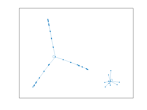
I'll turn it into a graph, so we can visualize what happens. It also gives me an excuse to employ a very pretty set of tools in MATLAB.
G2 = graph(N+1,Nmap+1,[],cellstr(dec2base(N,10,2)));
plot(G2)
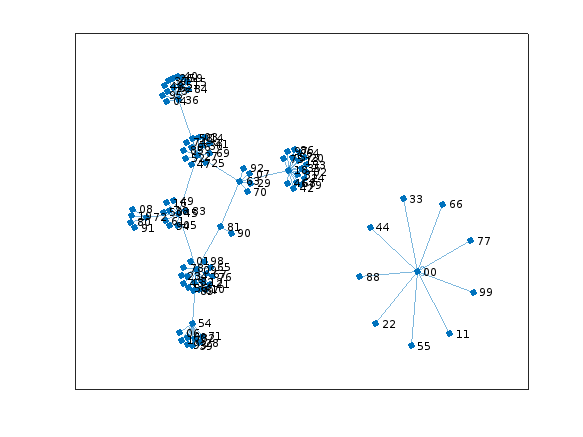
Do you see what happens? All of the rep-digit numbers, like 11, 44, 55, etc., all map directly to 0, and they stay there, since 0 also maps into 0. We can see that in the star on the lower right.
G2cycles = cyclebasis(G2)
G2cycles{1}
All other numbers eventually end up in the cycle:
G2cycles{2}
That is
81 ==> 63 ==> 27 ==> 45 ==> 09 ==> and back to 81
looping forever.
Another way of trying to visualize what happens with 2 digit numbers is to use symbolics. Thus, if we assume any 2 digit number can be written as 10*T+U, where I'll assume T>=U, since we always sort the digits first
syms T U
(10*T + U) - (10*U+T)
So after one iteration for 2 digit numbers, the result maps ALWAYS to a new 2 digit number that is divisible by 9. And there are only 10 such 2 digit numbers that are divisible by 9. So the 2-digit case must resolve itself rather quickly.
What happens when we move to 3 digit numbers? Note that for any 3 digit number abc (without loss of generality, assume a >= b >= c) it almost looks like it reduces to the 2 digit probem, aince we have abc - cba. The middle digit will always cancel itself in the subtraction operation. Does that mean we should expect a cycle at the end, as happens with 2 digit numbers? A simple modification to our previous code will tell us the answer.
N = (0:999)';
Ndig = dec2base(N,10,3) - '0';
Nmap = sort(Ndig,2,'descend')*[100;10;1] - sort(Ndig,2,'ascend')*[100;10;1];
G3 = graph(N+1,Nmap+1,[],cellstr(dec2base(N,10,2)));
plot(G3)
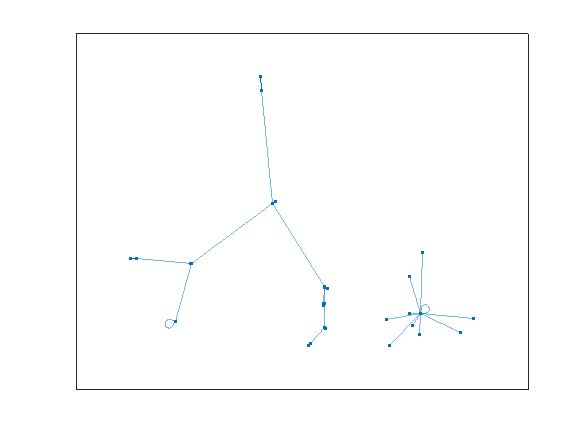
This one is more difficult to visualize, since there are 1000 nodes in the graph. However, we can clearly see two disjoint groups.
We can use cyclebasis to tell us the complete story again.
G3cycles = cyclebasis(G3)
G3cycles{:}
And we see that all 3 digit numbers must either terminate at 000, or 495. For example, if we start with 181, we would see:
811 - 118
963 - 369
954 - 459
It will terminate there, forever trapped at 495. And cyclebasis tells us there are no other cycles besides the boring one at 000.
What is the maximum length of any such path to get to 495?
D3 = distances(G3,496) % Remember, MATLAB uses an index origin of 1
D3(isinf(D3)) = -inf; % some nodes can never reach 495, so they have an infinite distance
plot(D3)
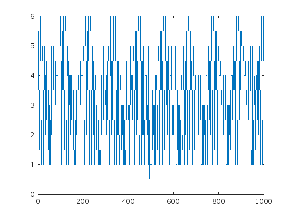
The maximum number of steps to get to 495 is 6 steps.
find(D3 == 6) - 1
So the 3 digit number 100 required 6 iterations to eventually reach 495.
shortestpath(G3,101,496) - 1
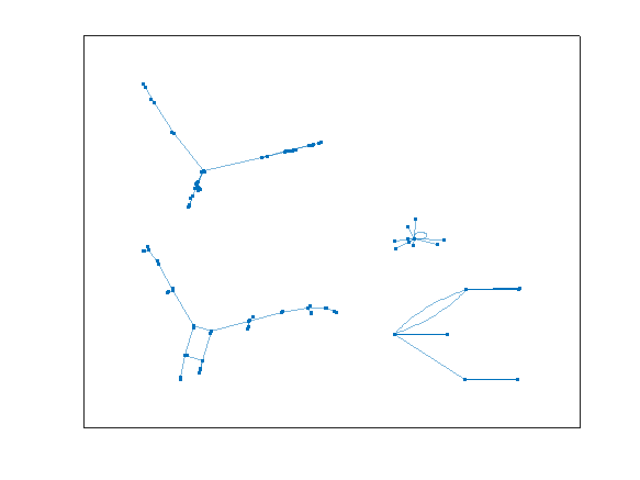
I think I've rather exhausted the 3 digit case. It is time now to move to the 4 digit problem, but we've already done all the hard work. The same scheme will apply to compute a graph. And the graph theory tools do all the hard work for us.
N = (0:9999)';
Ndig = dec2base(N,10,4) - '0';
Nmap = sort(Ndig,2,'descend')*[1000;100;10;1] - sort(Ndig,2,'ascend')*[1000;100;10;1];
G4 = graph(N+1,Nmap+1,[],cellstr(dec2base(N,10,2)));
plot(G4)
cyclebasis(G4)
ans{:}
And here we see the behavior, with one stable final point, 6174 as the only non-zero ending state. There are no circular cycles as we had for the 2-digit case.
How many iterations were necessary at most before termination?
D4 = distances(G4,6175);
D4(isinf(D4)) = -inf;
plot(D4)
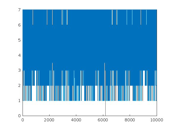
The plot tells the story here. The maximum number of iterations before termination is 7 for the 4 digit case.
find(D4 == 7,1,'last') - 1
shortestpath(G4,9986,6175) - 1
Can you go further? Are there 5 or 6 digit Kaprekar constants? Sadly, I have read that for more than 4 digits, things break down a bit, there is no 5 digit (or higher) Kaprekar constant.
We can verify that fact, at least for 5 digit numbers.
N = (0:99999)';
Ndig = dec2base(N,10,5) - '0';
Nmap = sort(Ndig,2,'descend')*[10000;1000;100;10;1] - sort(Ndig,2,'ascend')*[10000;1000;100;10;1];
G5 = graph(N+1,Nmap+1,[],cellstr(dec2base(N,10,2)));
plot(G5)
cyclebasis(G5)
ans{:}
The result here are 4 disjoint cycles. Of course the rep-digit cycle must always be on its own, but the other three cycles are also fully disjoint, and are of respective length 2, 4, and 4.
isequaln exists to return true when NaN==NaN.
unique treats NaN==NaN as false (as it should) requiring NaN to be replaced if NaN is not considered unique in a particular application. In my application, I am checking uniqueness of table rows using [table_unique,index_unique]=unique(table,"rows","sorted") and would prefer to keep NaN as NaN or missing in table_unique without the overhead of replacing it with a dummy value then replacing it again. Dummy values also have the risk of matching existing values in the table, requiring first finding a dummy value that is not in the table.
uniquen (similar to isequaln) would be more eloquent.
Please point out if I am missing something!
So generally I want to be using uifigures over figures. For example I really like the tab group component, which can really help with organizing large numbers of plots in a manageable way. I also really prefer the look of the progress dialog, uialert, confirm, etc. That said, I run into way more bugs using uifigures. I always get a “flicker” in the axes toolbar for example. I also have matlab getting “hung” a lot more often when using uifigures.
So in general, what is recommended? Are uifigures ever going to fully replace traditional figures? Are they going to become more and more robust? Do I need a better GPU to handle graphics better? Just looking for general guidance.
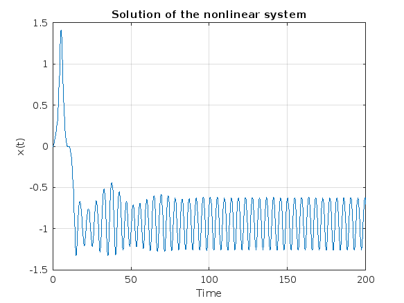
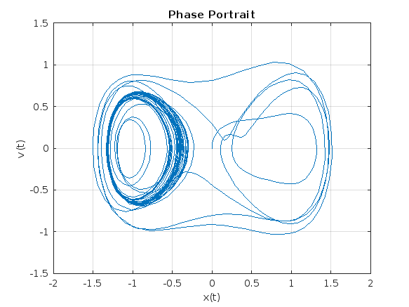
Following on from my previous post The Non-Chaotic Duffing Equation, now we will study the chaotic behaviour of the Duffing Equation
P.s:Any comments/advice on improving the code is welcome.
The Original Duffing Equation is the following:
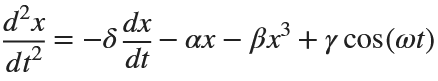
Let 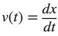 . This implies that
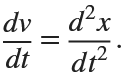
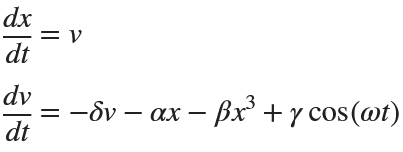
Then we rewrite it as a System of First-Order Equations
Using the substitution  for
for  , the second-order equation can be transformed into the following system of first-order equations:
Exploring the Effect of γ.
% Define parameters
gamma = 0.1;
alpha = -1;
beta = 1;
delta = 0.1;
omega = 1.4;
% Define the system of equations
odeSystem = @(t, y) [y(2);
-delta*y(2) - alpha*y(1) - beta*y(1)^3 + gamma*cos(omega*t)];
% Initial conditions
y0 = [0; 0]; % x(0) = 0, v(0) = 0
% Time span
tspan = [0 200];
% Solve the system
[t, y] = ode45(odeSystem, tspan, y0);
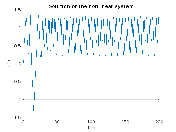
% Plot the results
figure;
plot(t, y(:, 1));
xlabel('Time');
ylabel('x(t)');
title('Solution of the nonlinear system');
grid on;
% Plot the phase portrait
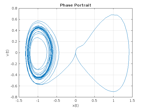
figure;
plot(y(:, 1), y(:, 2));
xlabel('x(t)');
ylabel('v(t)');
title('Phase Portrait');
grid on;
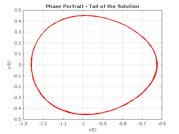
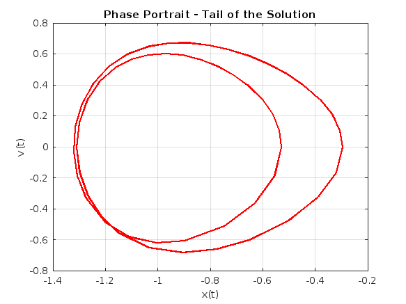
% Define the tail (e.g., last 10% of the time interval)
tail_start = floor(0.9 * length(t)); % Starting index for the tail
tail_end = length(t); % Ending index for the tail
% Plot the tail of the solution
figure;
plot(y(tail_start:tail_end, 1), y(tail_start:tail_end, 2), 'r', 'LineWidth', 1.5);
xlabel('x(t)');
ylabel('v(t)');
title('Phase Portrait - Tail of the Solution');
grid on;
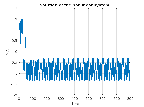
% Define parameters
gamma = 0.318;
alpha = -1;
beta = 1;
delta = 0.1;
omega = 1.4;
% Define the system of equations
odeSystem = @(t, y) [y(2);
-delta*y(2) - alpha*y(1) - beta*y(1)^3 + gamma*cos(omega*t)];
% Initial conditions
y0 = [0; 0]; % x(0) = 0, v(0) = 0
% Time span
tspan = [0 800];
% Solve the system
[t, y] = ode45(odeSystem, tspan, y0);
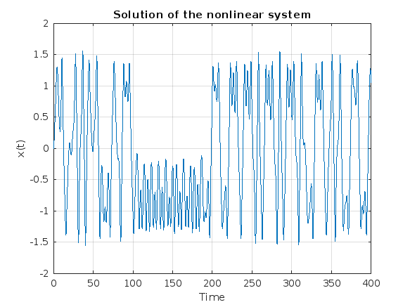
% Plot the results
figure;
plot(t, y(:, 1));
xlabel('Time');
ylabel('x(t)');
title('Solution of the nonlinear system');
grid on;
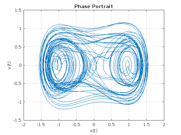
% Plot the phase portrait
figure;
plot(y(:, 1), y(:, 2));
xlabel('x(t)');
ylabel('v(t)');
title('Phase Portrait');
grid on;
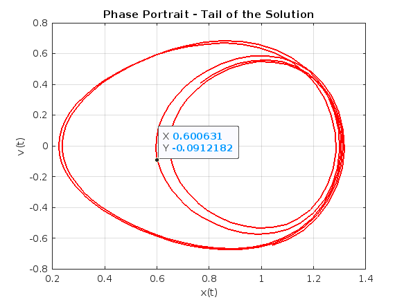
% Define the tail (e.g., last 10% of the time interval)
tail_start = floor(0.9 * length(t)); % Starting index for the tail
tail_end = length(t); % Ending index for the tail
% Plot the tail of the solution
figure;
plot(y(tail_start:tail_end, 1), y(tail_start:tail_end, 2), 'r', 'LineWidth', 1.5);
xlabel('x(t)');
ylabel('v(t)');
title('Phase Portrait - Tail of the Solution');
grid on;
% Define parameters
gamma = 0.338;
alpha = -1;
beta = 1;
delta = 0.1;
omega = 1.4;
% Define the system of equations
odeSystem = @(t, y) [y(2);
-delta*y(2) - alpha*y(1) - beta*y(1)^3 + gamma*cos(omega*t)];
% Initial conditions
y0 = [0; 0]; % x(0) = 0, v(0) = 0
% Time span with more points for better resolution
tspan = linspace(0, 200,2000); % Increase the number of points
% Solve the system
[t, y] = ode45(odeSystem, tspan, y0);
% Plot the results
figure;
plot(t, y(:, 1));
xlabel('Time');
ylabel('x(t)');
title('Solution of the nonlinear system');
grid on;
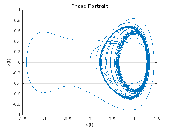
% Plot the phase portrait
figure;
plot(y(:, 1), y(:, 2));
xlabel('x(t)');
ylabel('v(t)');
title('Phase Portrait');
grid on;
% Define the tail (e.g., last 10% of the time interval)
tail_start = floor(0.9 * length(t)); % Starting index for the tail
tail_end = length(t); % Ending index for the tail
% Plot the tail of the solution
figure;
plot(y(tail_start:tail_end, 1), y(tail_start:tail_end, 2), 'r', 'LineWidth', 1.5);
xlabel('x(t)');
ylabel('v(t)');
title('Phase Portrait - Tail of the Solution');
grid on;
ax = gca;
chart = ax.Children(1);
datatip(chart,0.5581,-0.1126);
% Define parameters
gamma = 0.35;
alpha = -1;
beta = 1;
delta = 0.1;
omega = 1.4;
% Define the system of equations
odeSystem = @(t, y) [y(2);
-delta*y(2) - alpha*y(1) - beta*y(1)^3 + gamma*cos(omega*t)];
% Initial conditions
y0 = [0; 0]; % x(0) = 0, v(0) = 0
% Time span with more points for better resolution
tspan = linspace(0, 400,3000); % Increase the number of points
% Solve the system
[t, y] = ode45(odeSystem, tspan, y0);
% Plot the results
figure;
plot(t, y(:, 1));
xlabel('Time');
ylabel('x(t)');
title('Solution of the nonlinear system');
grid on;
% Plot the phase portrait
figure;
plot(y(:, 1), y(:, 2));
xlabel('x(t)');
ylabel('v(t)');
title('Phase Portrait');
grid on;
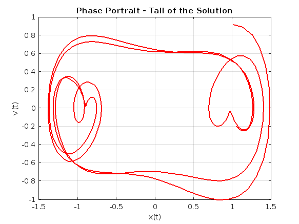
% Define the tail (e.g., last 10% of the time interval)
tail_start = floor(0.9 * length(t)); % Starting index for the tail
tail_end = length(t); % Ending index for the tail
% Plot the tail of the solution
figure;
plot(y(tail_start:tail_end, 1), y(tail_start:tail_end, 2), 'r', 'LineWidth', 1.5);
xlabel('x(t)');
ylabel('v(t)');
title('Phase Portrait - Tail of the Solution');
grid on;
Hi everyone, I am from India ..Suggest some drone for deploying code from Matlab.
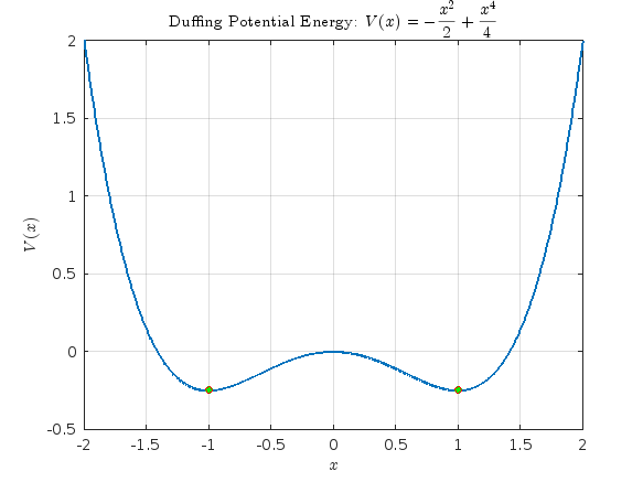
Studying the attached document Duffing Equation from the University of Colorado, I noticed that there is an analysis of The Non-Chaotic Duffing Equation and all the graphs were created with Matlab. And since the code is not given I took the initiative to try to create the same graphs with the following code.
- Plotting the Potential Energy and Identifying Extrema
% Define the range of x values
x = linspace(-2, 2, 1000);
% Define the potential function V(x)
V = -x.^2 / 2 + x.^4 / 4;
% Plot the potential function
figure;
plot(x, V, 'LineWidth', 2);
hold on;
% Mark the minima at x = ±1
plot([-1, 1], [-1/4, -1/4], 'ro', 'MarkerSize', 5, 'MarkerFaceColor', 'g');
% Add LaTeX title and labels
title('Duffing Potential Energy: $$V(x) = -\frac{x^2}{2} + \frac{x^4}{4}$$', 'Interpreter', 'latex');
xlabel('$$x$$', 'Interpreter', 'latex');
ylabel('$$V(x)$$','Interpreter', 'latex');
grid on;
hold off;
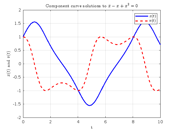
- Solving and Plotting the Duffing Equation
% Define the system of ODEs for the non-chaotic Duffing equation
duffing_ode = @(t, X) [X(2);
X(1) - X(1).^3];
% Time span for the simulation
tspan = [0 10];
% Initial conditions [x(0), v(0)]
initial_conditions = [1; 1];
% Solve the ODE using ode45
[t, X] = ode45(duffing_ode, tspan, initial_conditions);
% Extract displacement (x) and velocity (v)
x = X(:, 1);
v = X(:, 2);
% Plot both x(t) and v(t) in the same figure
figure;
plot(t, x, 'b-', 'LineWidth', 2); % Plot x(t) with blue line
hold on;
plot(t, v, 'r--', 'LineWidth', 2); % Plot v(t) with red dashed line
% Add title, labels, and legend
title(' Component curve solutions to $$\ddot{x}-x+x^3=0$$','Interpreter', 'latex');
xlabel('t','Interpreter', 'latex');
ylabel('$$x(t) $$ and $$v(t) $$','Interpreter', 'latex');
legend('$$x(t)$$', ' $$v(t)$$','Interpreter', 'latex');
grid on;
hold off;
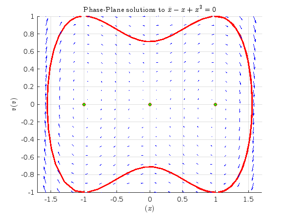
% Phase portrait with nullclines, equilibria, and vector field
figure;
hold on;
% Plot phase portrait
plot(x, v,'r', 'LineWidth', 2);
% Plot equilibrium points
plot([0 1 -1], [0 0 0], 'ro', 'MarkerSize', 5, 'MarkerFaceColor', 'g');
% Create a grid of points for the vector field
[x_vals, v_vals] = meshgrid(linspace(-2, 2, 20), linspace(-1, 1, 20));
% Compute the vector field components
dxdt = v_vals;
dvdt = x_vals - x_vals.^3;
% Plot the vector field
quiver(x_vals, v_vals, dxdt, dvdt, 'b');
% Set axis limits to [-1, 1]
xlim([-1.7 1.7]);
ylim([-1 1]);
% Labels and title
title('Phase-Plane solutions to $$\ddot{x}-x+x^3=0$$','Interpreter', 'latex');
xlabel('$$ (x)$$','Interpreter', 'latex');
ylabel('$$v(v)$$','Interpreter', 'latex');
grid on;
hold off;
Hello :-) I am interested in reading the book "The finite element method for solid and structural mechanics" online with somebody who is also interested in studying the finite element method particularly its mathematical aspect. I enjoy discussing the book instead of reading it alone. Please if you were interested email me at: student.z.k@hotmail.com Thank you!
An attractor is called strange if it has a fractal structure, that is if it has non-integer Hausdorff dimension. This is often the case when the dynamics on it are chaotic, but strange nonchaotic attractors also exist. If a strange attractor is chaotic, exhibiting sensitive dependence on initial conditions, then any two arbitrarily close alternative initial points on the attractor, after any of various numbers of iterations, will lead to points that are arbitrarily far apart (subject to the confines of the attractor), and after any of various other numbers of iterations will lead to points that are arbitrarily close together. Thus a dynamic system with a chaotic attractor is locally unstable yet globally stable: once some sequences have entered the attractor, nearby points diverge from one another but never depart from the attractor.
The term strange attractor was coined by David Ruelle and Floris Takens to describe the attractor resulting from a series of bifurcations of a system describing fluid flow. Strange attractors are often differentiable in a few directions, but some are like a Cantor dust, and therefore not differentiable. Strange attractors may also be found in the presence of noise, where they may be shown to support invariant random probability measures of Sinai–Ruelle–Bowen type.
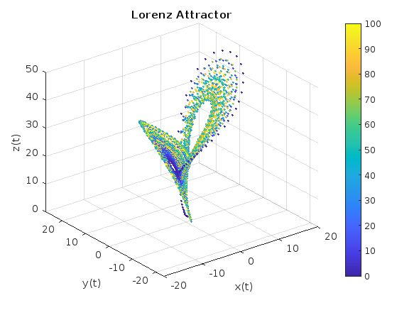
Lorenz
% Lorenz Attractor Parameters
sigma = 10;
beta = 8/3;
rho = 28;
% Lorenz system of differential equations
f = @(t, a) [-sigma*a(1) + sigma*a(2);
rho*a(1) - a(2) - a(1)*a(3);
-beta*a(3) + a(1)*a(2)];
% Time span
tspan = [0 100];
% Initial conditions
a0 = [1 1 1];
% Solve the system using ode45
[t, a] = ode45(f, tspan, a0);
% Plot using scatter3 with time-based color mapping
figure;
scatter3(a(:,1), a(:,2), a(:,3), 5, t, 'filled'); % 5 is the marker size
title('Lorenz Attractor');
xlabel('x(t)');
ylabel('y(t)');
zlabel('z(t)');
grid on;
colorbar; % Add a colorbar to indicate the time mapping
view(3); % Set the view to 3D
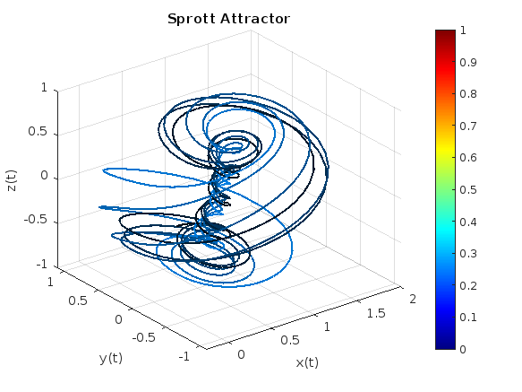
Sprott
% Define the parameters
a = 2.07;
b = 1.79;
% Define the system of differential equations
dynamics = @(t, X) [ ...
X(2) + a * X(1) * X(2) + X(1) * X(3); % dx/dt
1 - b * X(1)^2 + X(2) * X(3); % dy/dt
X(1) - X(1)^2 - X(2)^2 % dz/dt
];
% Initial conditions
X0 = [0.63; 0.47; -0.54];
% Time span
tspan = [0 100];
% Solve the system using ode45
[t, X] = ode45(dynamics, tspan, X0);
% Plot the results with color gradient
figure;
colormap(jet); % Set the colormap
c = linspace(1, 10, length(t)); % Color data based on time
% Create a 3D line plot with color based on time
for i = 1:length(t)-1
plot3(X(i:i+1,1), X(i:i+1,2), X(i:i+1,3), 'Color', [0 0.5 0.9]*c(i)/10, 'LineWidth', 1.5);
hold on;
end
% Set plot properties
title('Sprott Attractor');
xlabel('x(t)');
ylabel('y(t)');
zlabel('z(t)');
grid on;
colorbar; % Add a colorbar to indicate the time mapping
view(3); % Set the view to 3D
hold off;
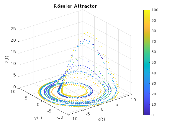
Rössler
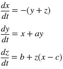
% Define the parameters
a = 0.2;
b = 0.2;
c = 5.7;
% Define the system of differential equations
dynamics = @(t, X) [ ...
-(X(2) + X(3)); % dx/dt
X(1) + a * X(2); % dy/dt
b + X(3) * (X(1) - c) % dz/dt
];
% Initial conditions
X0 = [10.0; 0.00; 10.0];
% Time span
tspan = [0 100];
% Solve the system using ode45
[t, X] = ode45(dynamics, tspan, X0);
% Plot the results
figure;
scatter3(X(:,1), X(:,2), X(:,3), 5, t, 'filled');
title('Rössler Attractor');
xlabel('x(t)');
ylabel('y(t)');
zlabel('z(t)');
grid on;
colorbar; % Add a colorbar to indicate the time mapping
view(3); % Set the view to 3D
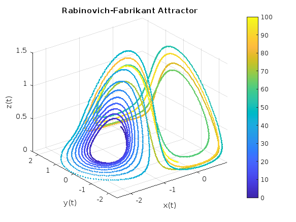
Rabinovich-Fabrikant
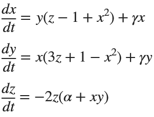
%% Parameters for Rabinovich-Fabrikant Attractor
alpha = 0.14;
gamma = 0.10;
dt = 0.01;
num_steps = 5000;
% Initial conditions
x0 = -1;
y0 = 0;
z0 = 0.5;
% Preallocate arrays for performance
x = zeros(1, num_steps);
y = zeros(1, num_steps);
z = zeros(1, num_steps);
% Set initial values
x(1) = x0;
y(1) = y0;
z(1) = z0;
% Generate the attractor
for i = 1:num_steps-1
x(i+1) = x(i) + dt * (y(i)*(z(i) - 1 + x(i)^2) + gamma*x(i));
y(i+1) = y(i) + dt * (x(i)*(3*z(i) + 1 - x(i)^2) + gamma*y(i));
z(i+1) = z(i) + dt * (-2*z(i)*(alpha + x(i)*y(i)));
end
% Create a time vector for color mapping
t = linspace(0, 100, num_steps);
% Plot using scatter3
figure;
scatter3(x, y, z, 5, t, 'filled'); % 5 is the marker size
title('Rabinovich-Fabrikant Attractor');
xlabel('x(t)');
ylabel('y(t)');
zlabel('z(t)');
grid on;
colorbar; % Add a colorbar to indicate the time mapping
view(3); % Set the view to 3D
References
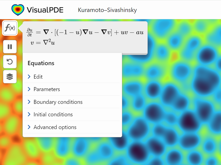
A library of runnable PDEs. See the equations! Modify the parameters! Visualize the resulting system in your browser! Convenient, fast, and instructive.
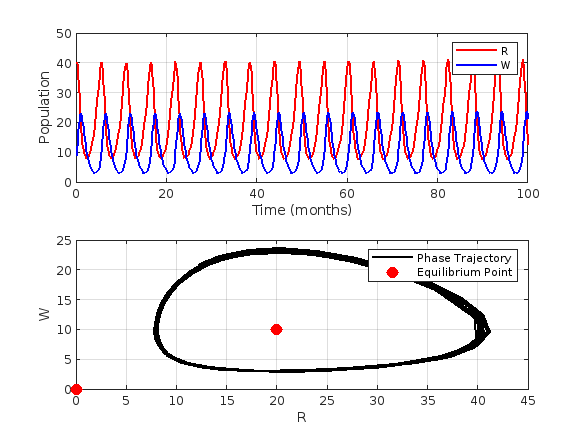
This project discusses predator-prey system, particularly the Lotka-Volterra equations,which model the interaction between two sprecies: prey and predators. Let's solve the Lotka-Volterra equations numerically and visualize the results.% Define parameters
% Define parameters
alpha = 1.0; % Prey birth rate
beta = 0.1; % Predator success rate
gamma = 1.5; % Predator death rate
delta = 0.075; % Predator reproduction rate
% Define the symbolic variables
syms R W
% Define the equations
eq1 = alpha * R - beta * R * W == 0;
eq2 = delta * R * W - gamma * W == 0;
% Solve the equations
equilibriumPoints = solve([eq1, eq2], [R, W]);
% Extract the equilibrium point values
Req = double(equilibriumPoints.R);
Weq = double(equilibriumPoints.W);
% Display the equilibrium points
equilibriumPointsValues = [Req, Weq]
% Solve the differential equations using ode45
lotkaVolterra = @(t,Y)[alpha*Y(1)-beta*Y(1)*Y(2);
delta*Y(1)*Y(2)-gamma*Y(2)];
% Initial conditions
R0 = 40;
W0 = 9;
Y0 = [R0, W0];
tspan = [0, 100];
% Solve the differential equations
[t, Y] = ode45(lotkaVolterra, tspan, Y0);
% Extract the populations
R = Y(:, 1);
W = Y(:, 2);
% Plot the results
figure;
subplot(2,1,1);
plot(t, R, 'r', 'LineWidth', 1.5);
hold on;
plot(t, W, 'b', 'LineWidth', 1.5);
xlabel('Time (months)');
ylabel('Population');
legend('R', 'W');
grid on;
subplot(2,1,2);
plot(R, W, 'k', 'LineWidth', 1.5);
xlabel('R');
ylabel('W');
grid on;
hold on;
plot(Req, Weq, 'ro', 'MarkerSize', 8, 'MarkerFaceColor', 'r');
legend('Phase Trajectory', 'Equilibrium Point');
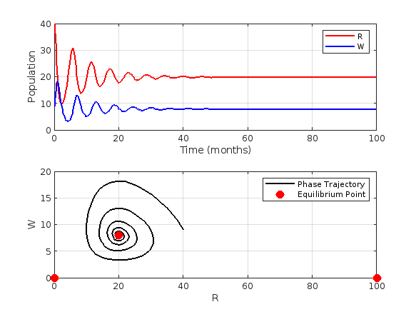
Now, we need to handle a modified version of the Lotka-Volterra equations. These modified equations incorporate logistic growth fot the prey population.
These equations are:
% Define parameters
alpha = 1.0;
K = 100; % Carrying Capacity of the prey population
beta = 0.1;
gamma = 1.5;
delta = 0.075;
% Define the symbolic variables
syms R W
% Define the equations
eq1 = alpha*R*(1 - R/K) - beta*R*W == 0;
eq2 = delta*R*W - gamma*W == 0;
% Solve the equations
equilibriumPoints = solve([eq1, eq2], [R, W]);
% Extract the equilibrium point values
Req = double(equilibriumPoints.R);
Weq = double(equilibriumPoints.W);
% Display the equilibrium points
equilibriumPointsValues = [Req, Weq]
% Solve the differential equations using ode45
modified_lv = @(t,Y)[alpha*Y(1)*(1-Y(1)/K)-beta*Y(1)*Y(2);
delta*Y(1)*Y(2)-gamma*Y(2)];
% Initial conditions
R0 = 40;
W0 = 9;
Y0 = [R0, W0];
tspan = [0, 100];
% Solve the differential equations
[t, Y] = ode45(modified_lv, tspan, Y0);
% Extract the populations
R = Y(:, 1);
W = Y(:, 2);
% Plot the results
figure;
subplot(2,1,1);
plot(t, R, 'r', 'LineWidth', 1.5);
hold on;
plot(t, W, 'b', 'LineWidth', 1.5);
xlabel('Time (months)');
ylabel('Population');
legend('R', 'W');
grid on;
subplot(2,1,2);
plot(R, W, 'k', 'LineWidth', 1.5);
xlabel('R');
ylabel('W');
grid on;
hold on;
plot(Req, Weq, 'ro', 'MarkerSize', 8, 'MarkerFaceColor', 'r');
legend('Phase Trajectory', 'Equilibrium Point');
Does your company or organization require that all your Word Documents and Excel workbooks be labeled with a Microsoft Azure Information Protection label or else they can't be saved? These are the labels that are right below the tool ribbon that apply a category label such as "Public", "Business Use", or "Highly Restricted". If so, you can either
- Create and save a "template file" with the desired label and then call copyfile to make a copy of that file and then write your results to the new copy, or
- If using Windows you can create and/or open the file using ActiveX and then apply the desired label from your MATLAB program's code.
For #1 you can do
copyfile(templateFileName, newDataFileName);
writematrix(myData, newDataFileName);
If the template has the AIP label applied to it, then the copy will also inherit the same label.
For #2, here is a demo for how to apply the code using ActiveX.
% Test to set the Microsoft Azure Information Protection label on an Excel workbook.
% Reference support article:
% https://www.mathworks.com/matlabcentral/answers/1901140-why-does-azure-information-protection-popup-pause-the-matlab-script-when-i-use-actxserver?s_tid=ta_ans_results
clc; % Clear the command window.
close all; % Close all figures (except those of imtool.)
clear; % Erase all existing variables. Or clearvars if you want.
workspace; % Make sure the workspace panel is showing.
format compact;
% Define your workbook file name.
excelFullFileName = fullfile(pwd, '\testAIP.xlsx');
% Make sure it exists. Open Excel as an ActiveX server if it does.
if isfile(excelFullFileName)
% If the workbook exists, launch Excel as an ActiveX server.
Excel = actxserver('Excel.Application');
Excel.visible = true; % Make the server visible.
fprintf('Excel opened successfully.\n');
fprintf('Your workbook file exists:\n"%s".\nAbout to try to open it.\n', excelFullFileName);
% Open up the existing workbook named in the variable fullFileName.
Excel.Workbooks.Open(excelFullFileName);
fprintf('Excel opened file successfully.\n');
else
% File does not exist. Alert the user.
warningMessage = sprintf('File does not exist:\n\n"%s"\n', excelFullFileName);
fprintf('%s\n', warningMessage);
errordlg(warningMessage);
return;
end
% If we get here, the workbook file exists and has been opened by Excel.
% Ask Excel for the Microsoft Azure Information Protection (AIP) label of the workbook we just opened.
label = Excel.ActiveWorkbook.SensitivityLabel.GetLabel
% See if there is a label already. If not, these will be null:
existingLabelID = label.LabelId
existingLabelName = label.LabelName
% Create a label.
label = Excel.ActiveWorkbook.SensitivityLabel.CreateLabelInfo
label.LabelId = "a518e53f-798e-43aa-978d-c3fda1f3a682";
label.LabelName = "Business Use";
% Assign the label to the workbook.
fprintf('Setting Microsoft Azure Information Protection to "Business Use", GUID of a518e53f-798e-43aa-978d-c3fda1f3a682\n');
Excel.ActiveWorkbook.SensitivityLabel.SetLabel(label, label);
% Save this workbook with the new AIP setting we just created.
Excel.ActiveWorkbook.Save;
% Shut down Excel.
Excel.ActiveWorkbook.Close;
Excel.Quit;
% Excel is now closed down. Delete the variable from the MATLAB workspace.
clear Excel;
% Now check to see if the AIP label has been set
% by opening up the file in Excel and looking at the AIP banner.
winopen(excelFullFileName)
Note that there is a line in there that gets an AIP label from the existing workbook, if there is one at all. If there is not one, you can set one. But to determine what the proper LabelId (that crazy long hexadecimal number) should be, you will probably need to open an existing document that already has the label that you want set (applied to it) and then read that label with this line:
label = Excel.ActiveWorkbook.SensitivityLabel.GetLabel
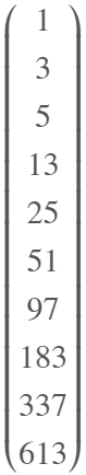
This stems purely from some play on my part. Suppose I asked you to work with the sequence formed as 2*n*F_n + 1, where F_n is the n'th Fibonacci number? Part of me would not be surprised to find there is nothing simple we could do. But, then it costs nothing to try, to see where MATLAB can take me in an explorative sense.
n = sym(0:100).';
Fn = fibonacci(n);
Sn = 2*n.*Fn + 1;
Sn(1:10) % A few elements
For kicks, I tried asking ChatGPT. Giving it nothing more than the first 20 members of thse sequence as integers, it decided this is a Perrin sequence, and gave me a recurrence relation, but one that is in fact incorrect. Good effort from the Ai, but a fail in the end.
Is there anything I can do? Try null! (Look carefully at the array generated by Toeplitz. It is at least a pretty way to generate the matrix I needed.)
X = toeplitz(Sn,[1,zeros(1,4)]);
rank(X(5:end,:))
Hmm. So there is no linear combination of those columns that yields all zeros, since the resulting matrix was full rank.
X = toeplitz(Sn,[1,zeros(1,5)]);
rank(X(6:end,:))
But if I take it one step further, we see the above matrix is now rank deficient. What does that tell me? It says there is some simple linear combination of the columns of X(6:end,:) that always yields zero. The previous test tells me there is no shorter constant coefficient recurrence releation, using fewer terms.
null(X(6:end,:))
Let me explain what those coefficients tell me. In fact, they yield a very nice recurrence relation for the sequence S_n, not unlike the original Fibonacci sequence it was based upon.
S(n+1) = 3*S(n) - S_(n-1) - 3*S(n-2) + S(n-3) + S(n-4)
where the first 5 members of that sequence are given as [1 3 5 13 25]. So a 6 term linear constant coefficient recurrence relation. If it reminds you of the generating relation for the Fibonacci sequence, that is good, because it should. (Remember I started the sequence at n==0, IF you decide to test it out.) We can test it out, like this:
SfunM = memoize(@(N) Sfun(N));
SfunM(25)
2*25*fibonacci(sym(25)) + 1
And indeed, it works as expected.
function Sn = Sfun(n)
switch n
case 0
Sn = 1;
case 1
Sn = 3;
case 2
Sn = 5;
case 3
Sn = 13;
case 4
Sn = 25;
otherwise
Sn = Sfun(n-5) + Sfun(n-4) - 3*Sfun(n-3) - Sfun(n-2) +3*Sfun(n-1);
end
end
A beauty of this, is I started from nothing but a sequence of integers, derived from an expression where I had no rational expectation of finding a formula, and out drops something pretty. I might call this explorational mathematics.
The next step of course is to go in the other direction. That is, given the derived recurrence relation, if I substitute the formula for S_n in terms of the Fibonacci numbers, can I prove it is valid in general? (Yes.) After all, without some proof, it may fail for n larger than 100. (I'm not sure how much I can cram into a single discussion, so I'll stop at this point for now. If I see interest in the ideas here, I can proceed further. For example, what was I doing with that sequence in the first place? And of course, can I prove the relation is valid? Can I do so using MATLAB?)
(I'll be honest, starting from scratch, I'm not sure it would have been obvious to find that relation, so null was hugely useful here.)
Hi everyone,
I've recently joined a forest protection team in Greece, where we use drones for various tasks. This has sparked my interest in drone programming, and I'd like to learn more about it. Can anyone recommend any beginner-friendly courses or programs that teach drone programming?
I'm particularly interested in courses that focus on practical applications and might align with the work we do in forest protection. Any suggestions or guidance would be greatly appreciated!
Thank you!
I have picked the title but don't know which direction to take it. Looking for any and all inspiration. I took the project as it sounded interesting when reading into it, but I'm a satellite novice, and my degree is in electronics.
"What are your favorite features or functionalities in MATLAB, and how have they positively impacted your projects or research? Any tips or tricks to share?
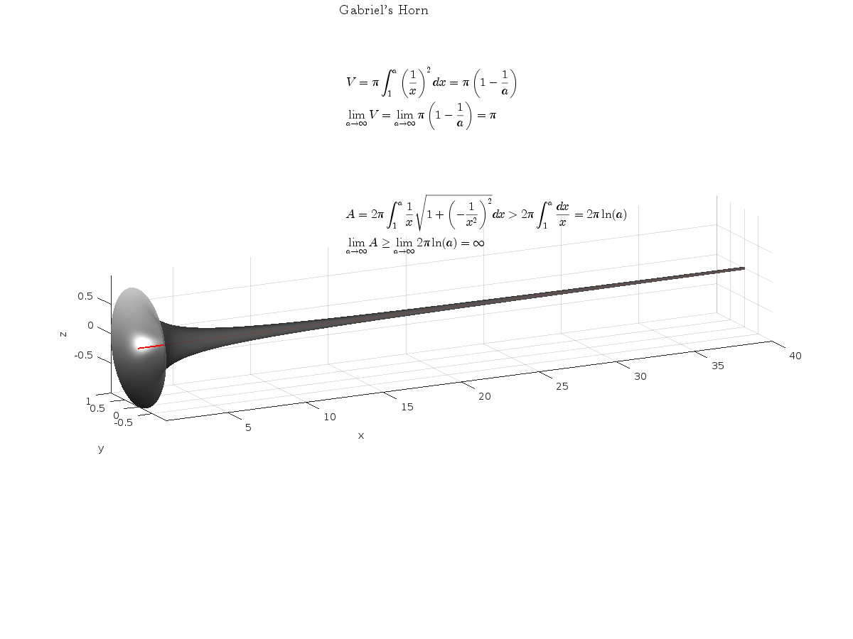
Gabriel's horn is a shape with the paradoxical property that it has infinite surface area, but a finite volume.
Gabriel’s horn is formed by taking the graph of  with the domain
  and rotating it in three dimensions about the
  axis.
axis.
There is a standard formula for calculating the volume of this shape, for a general function  .Wwe will just state that the volume of the
  solid between a and b is:
The surface area of the solid is given by:
One other thing we need to consider is that we are trying to find the value of these integrals between 1 and ∞. An integral with a limit of infinity is called an improper integral and we can't evaluate it simply by plugging the value infinity into the normal equation for a definite integral. Instead, we must first calculate the definite integral up to some finite limit b and then calculate the limit of the result as b tends to ∞:
Volume
We can calculate the horn's volume using the volume integral above, so
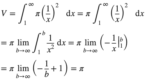
The total volume of this infinitely long trumpet isπ.
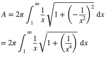
Surface Area
To determine the surface area, we first need the function’s derivative:
Now plug it into the surface area formula and we have:
This is an improper integral and it's hard to evaluate, but since in our interval 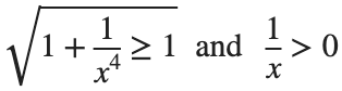
So, we have :
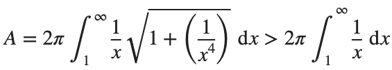
Now,we evaluate this last integral
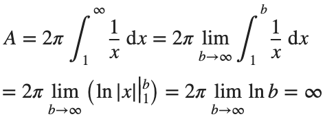
So the surface are is infinite.
% Define the function for Gabriel's Horn
gabriels_horn = @(x) 1 ./ x;
% Create a range of x values
x = linspace(1, 40, 4000); % Increase the number of points for better accuracy
y = gabriels_horn(x);
% Create the meshgrid
theta = linspace(0, 2 * pi, 6000); % Increase theta points for a smoother surface
[X, T] = meshgrid(x, theta);
Y = gabriels_horn(X) .* cos(T);
Z = gabriels_horn(X) .* sin(T);
% Plot the surface of Gabriel's Horn
figure('Position', [200, 100, 1200, 900]);
surf(X, Y, Z, 'EdgeColor', 'none', 'FaceAlpha', 0.9);
hold on;
% Plot the central axis
plot3(x, zeros(size(x)), zeros(size(x)), 'r', 'LineWidth', 2);
% Set labels
xlabel('x');
ylabel('y');
zlabel('z');
% Adjust colormap and axis properties
colormap('gray');
shading interp; % Smooth shading
% Adjust the view
view(3);
axis tight;
grid on;
% Add formulas as text annotations
dim1 = [0.4 0.7 0.3 0.2];
annotation('textbox',dim1,'String',{'$$V = \pi \int_{1}^{a} \left( \frac{1}{x} \right)^2 dx = \pi \left( 1 - \frac{1}{a} \right)$$', ...
'', ... % Add an empty line for larger gap
'$$\lim_{a \to \infty} V = \lim_{a \to \infty} \pi \left( 1 - \frac{1}{a} \right) = \pi$$'}, ...
'Interpreter','latex','FontSize',12, 'EdgeColor','none', 'FitBoxToText', 'on');
dim2 = [0.4 0.5 0.3 0.2];
annotation('textbox',dim2,'String',{'$$A = 2\pi \int_{1}^{a} \frac{1}{x} \sqrt{1 + \left( -\frac{1}{x^2} \right)^2} dx > 2\pi \int_{1}^{a} \frac{dx}{x} = 2\pi \ln(a)$$', ...
'', ... % Add an empty line for larger gap
'$$\lim_{a \to \infty} A \geq \lim_{a \to \infty} 2\pi \ln(a) = \infty$$'}, ...
'Interpreter','latex','FontSize',12, 'EdgeColor','none', 'FitBoxToText', 'on');
% Add Gabriel's Horn label
dim3 = [0.3 0.9 0.3 0.1];
annotation('textbox',dim3,'String','Gabriel''s Horn', ...
'Interpreter','latex','FontSize',14, 'EdgeColor','none', 'HorizontalAlignment', 'center');
hold off
daspect([3.5 1 1]) % daspect([x y z])
view(-27, 15)
lightangle(-50,0)
lighting('gouraud')
The properties of this figure were first studied by Italian physicist and mathematician Evangelista Torricelli in the 17th century.
Acknowledgment
I would like to express my sincere gratitude to all those who have supported and inspired me throughout this project.
First and foremost, I would like to thank the mathematician and my esteemed colleague, Stavros Tsalapatis, for inspiring me with the fascinating subject of Gabriel's Horn.
I am also deeply thankful to Mr. @Star Strider for his invaluable assistance in completing the final code.
References:
您也可以从以下列表中选择网站:
美洲
- América Latina (Español)
- Canada (English)
- United States (English)
欧洲
- Belgium (English)
- Denmark (English)
- Deutschland (Deutsch)
- España (Español)
- Finland (English)
- France (Français)
- Ireland (English)
- Italia (Italiano)
- Luxembourg (English)
- Netherlands (English)
- Norway (English)
- Österreich (Deutsch)
- Portugal (English)
- Sweden (English)
- Switzerland
- United Kingdom(English)
亚太
- Australia (English)
- India (English)
- New Zealand (English)
- 中国
- 日本Japanese (日本語)
- 한국Korean (한국어)