主要内容
搜索
Local large language models (LLMs), such as llama, phi3, and mistral, are now available in the Large Language Models (LLMs) with MATLAB repository through Ollama™!
Read about it here:
As far as I know, starting from MATLAB R2024b, the documentation is defaulted to be accessed online. However, the problem is that every time I open the official online documentation through my browser, it defaults or forcibly redirects to the documentation hosted site for my current geographic location, often with multiple pop-up reminders, which is very annoying!
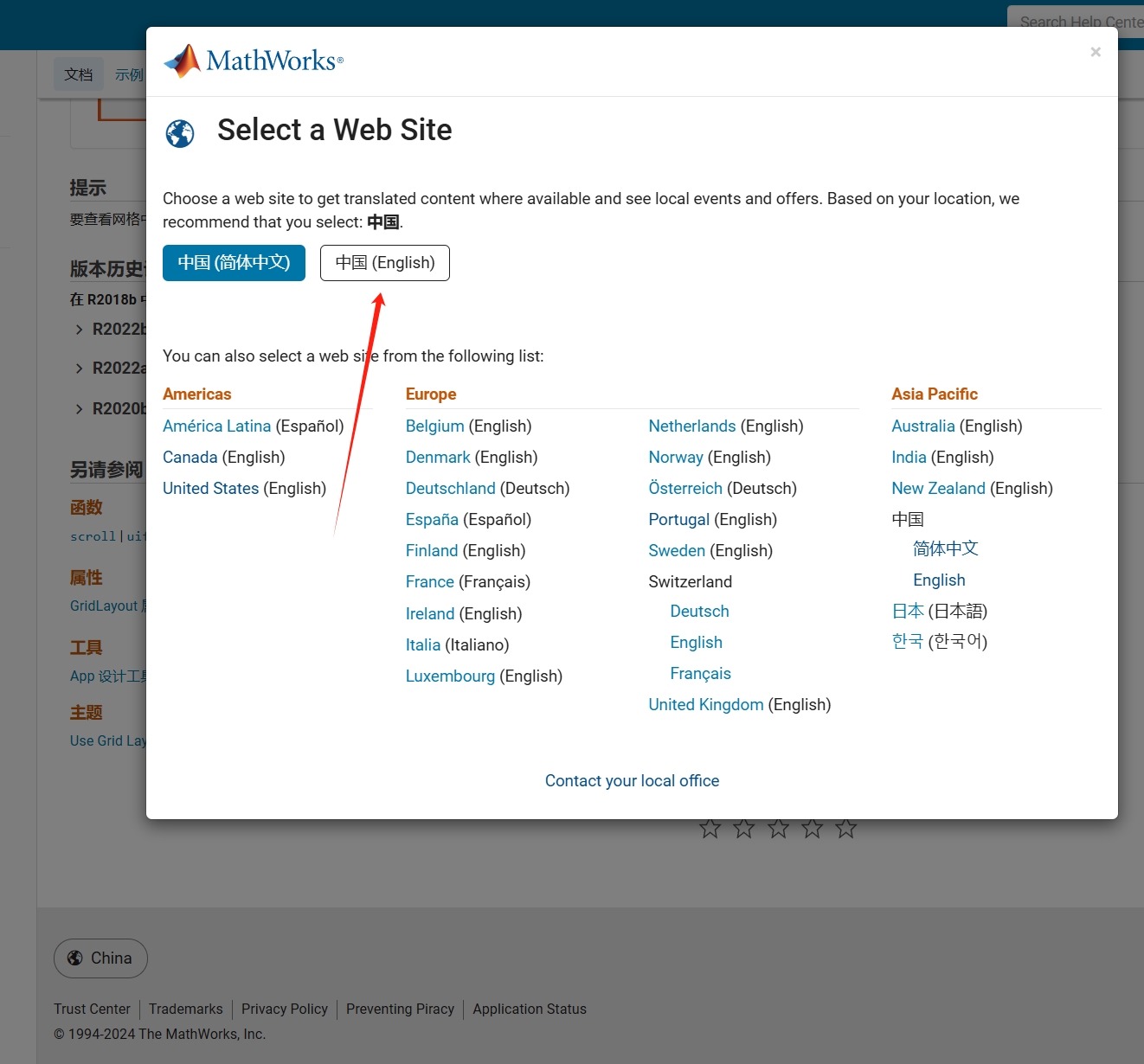
Suggestion: Could there be an option to set preferences linked to my personal account so that the documentation defaults to my chosen language preference without having to deal with “forced reminders” or “forced redirection” based on my geographic location? I prefer reading the English documentation, but the website automatically redirects me to the Chinese documentation due to my geolocation, which is quite frustrating!
----------------2024.12.13 update-----------------
Although the above issue was resolved by technical support, subsequent redirects are still causing severe delays...
In the past two years, MATHWORKS has updated the image viewer and audio viewer, giving them a more modern interface with features like play, pause, fast forward, and some interactive tools that are more commonly found in typical third-party players. However, the video player has not seen any updates. For instance, the Video Viewer or vision.VideoPlayer could benefit from a more modern player interface. Perhaps I haven't found a suitable built-in player yet. It would be great if there were support for custom image processing and audio processing algorithms that could be played in a more modern interface in real time.
Additionally, I found it quite challenging to develop a modern video player from scratch in App Designer.(If there's a video component for that that would be great)
-----------------------------------------------------------------------------------------------------------------
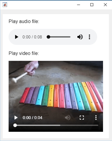
BTW,the following picture shows the built-in function uihtml function showing a more modern playback interface with controls for play, pause and so on. But can not add real-time image processing algorithms within it.
I was browsing the MathWorks website and decided to check the Cody leaderboard. To my surprise, William has now solved 5,000 problems. At the moment, there are 5,227 problems on Cody, so William has solved over 95%. The next competitor is over 500 problems behind. His score is also clearly the highest, approaching 60,000.
I've been working on some matrix problems recently(Problem 55225)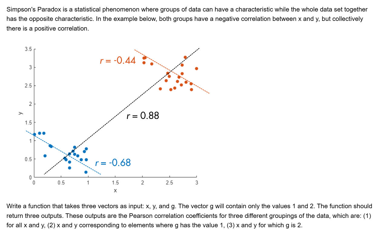
and this is my code
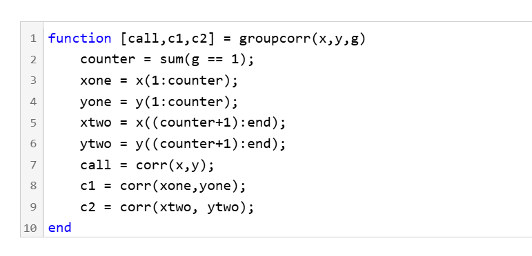
It turns out that "Undefined function 'corr' for input arguments of type 'double'." However, should't the input argument of "corr" be column vectors with single/double values? What's even going on there?
isequaln exists to return true when NaN==NaN.
unique treats NaN==NaN as false (as it should) requiring NaN to be replaced if NaN is not considered unique in a particular application. In my application, I am checking uniqueness of table rows using [table_unique,index_unique]=unique(table,"rows","sorted") and would prefer to keep NaN as NaN or missing in table_unique without the overhead of replacing it with a dummy value then replacing it again. Dummy values also have the risk of matching existing values in the table, requiring first finding a dummy value that is not in the table.
uniquen (similar to isequaln) would be more eloquent.
Please point out if I am missing something!
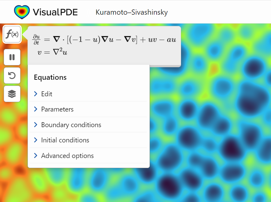
A library of runnable PDEs. See the equations! Modify the parameters! Visualize the resulting system in your browser! Convenient, fast, and instructive.
hello i found the following tools helpful to write matlab programs. copilot.microsoft.com chatgpt.com/gpts gemini.google.com and ai.meta.com. thanks a lot and best wishes.
Hi everyone,
I've recently joined a forest protection team in Greece, where we use drones for various tasks. This has sparked my interest in drone programming, and I'd like to learn more about it. Can anyone recommend any beginner-friendly courses or programs that teach drone programming?
I'm particularly interested in courses that focus on practical applications and might align with the work we do in forest protection. Any suggestions or guidance would be greatly appreciated!
Thank you!
"What are your favorite features or functionalities in MATLAB, and how have they positively impacted your projects or research? Any tips or tricks to share?
Check out the LLMs with MATLAB project on File Exchange to access Large Language Models from MATLAB.
Along with the latest support for GPT-4o mini, you can use LLMs with MATLAB to generate images, categorize data, and provide semantic analyis.
function ans = your_fcn_name(n)
n;
j=sum(1:n);
a=zeros(1,j);
for i=1:n
a(1,((sum(1:(i-1))+1)):(sum(1:(i-1))+i))=i.*ones(1,i);
end
disp
I am trying to earn my Intro to MATLAB badge in Cody, but I cannot click the Roll the Dice! problem. It simply is not letting me click it, therefore I cannot earn my badge. Does anyone know who I should contact or what to do?
Something that had bothered me ever since I became an FEA analyst (2012) was the apparent inability of the "camera" in Matlab's 3D plot to function like the "cameras" in CAD/CAE packages.
For instance, load the ForearmLink.stl model that ships with the PDE Toolbox in Matlab and ParaView and try rotating the model.
clear
close all
gm = importGeometry( "ForearmLink.stl" );
pdegplot(gm)
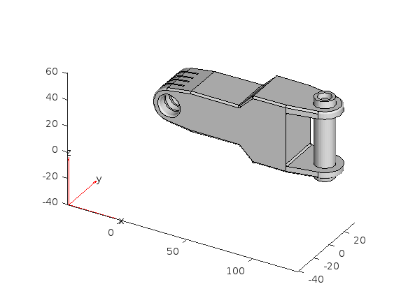
Things to observe:
- Note that I cant seem to rotate continuously around the x-axis. It appears to only support rotations from [0, 360] as opposed to [-inf, inf]. So, for example, if I'm looking in the Y+ direction and rotate around X so that I'm looking at the Z- direction, and then want to look in the Y- direction, I can't simply keep rotating around the X axis... instead have to rotate 180 degrees around the Z axis and then around the X axis. I'm not aware of any data visualization applications (e.g., ParaView, VisIt, EnSight) or CAD/CAE tools with such an interaction.
- Note that at the 50 second mark, I set a view in ParaView: looking in the [X-, Y-, Z-] direction with Y+ up. Try as I might in Matlab, I'm unable to achieve that same view perspective.
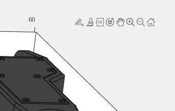
Today I discovered that if one turns on the Camera Toolbar from the View menubar, then clicks the Orbit Camera icon, then the No Principal Axis icon:
That then it acts in the manner I've long desired. Oh, and also, for the interested, it is programmatically available: https://www.mathworks.com/help/matlab/ref/cameratoolbar.html
I might humbly propose this mode either be made more discoverable, similar to the little interaction widgets that pop up in figures:
Or maybe use the middle-mouse button to temporarily use this mode (a mouse setting in, e.g., Abaqus/CAE).
I've noticed is that the highly rated fonts for coding (e.g. Fira Code, Inconsolata, etc.) seem to overlook one issue that is key for coding in Matlab. While these fonts make 0 and O, as well as the 1 and l easily distinguishable, the brackets are not. Quite often the curly bracket looks similar to the curved bracket, which can lead to mistakes when coding or reviewing code.
So I was thinking: Could Mathworks put together a team to review good programming fonts, and come up with their own custom font designed specifically and optimized for Matlab syntax?
An option for 10th degree polynomials but no weighted linear least squares. Seriously? Jesse
What do you think about the NVIDIA's achivement of becoming the top giant of manufacturing chips, especially for AI world?

Twitch built an entire business around letting you watch over someone's shoulder while they play video games. I feel like we should be able to make at least a few videos where we get to watch over someone's shoulder while they solve Cody problems. I would pay good money for a front-row seat to watch some of my favorite solvers at work. Like, I want to know, did Alfonso Nieto-Castonon just sit down and bang out some of those answers, or did he have to think about it for a while? What was he thinking about while he solved it? What resources was he drawing on? There's nothing like watching a master craftsman at work.
I can imagine a whole category of Cody videos called "How I Solved It". I tried making one of these myself a while back, but as far as I could tell, nobody else made one.
Here's the direct link to the video: https://www.youtube.com/watch?v=hoSmO1XklAQ
I hereby challenge you to make a "How I Solved It" video and post it here. If you make one, I'll make another one.
The Ans Hack is a dubious way to shave a few points off your solution score. Instead of a standard answer like this
function y = times_two(x)
y = 2*x;
end
you would do this
function ans = times_two(x)
2*x;
end
The ans variable is automatically created when there is no left-hand side to an evaluated expression. But it makes for an ugly function. I don't think anyone actually defends it as a good practice. The question I would ask is: is it so offensive that it should be specifically disallowed by the rules? Or is it just one of many little hacks that you see in Cody, inelegant but tolerable in the context of the surrounding game?
Incidentally, I wrote about the Ans Hack long ago on the Community Blog. Dealing with user-unfriendly code is also one of the reasons we created the Head-to-Head voting feature. Some techniques are good for your score, and some are good for your code readability. You get to decide with you care about.
There are a host of problems on Cody that require manipulation of the digits of a number. Examples include summing the digits of a number, separating the number into its powers, and adding very large numbers together.
If you haven't come across this trick yet, you might want to write it down (or save it electronically):
digits = num2str(4207) - '0'
That code results in the following:
digits =
4 2 0 7
Now, summing the digits of the number is easy:
sum(digits)
ans =
13
您也可以从以下列表中选择网站:
美洲
- América Latina (Español)
- Canada (English)
- United States (English)
欧洲
- Belgium (English)
- Denmark (English)
- Deutschland (Deutsch)
- España (Español)
- Finland (English)
- France (Français)
- Ireland (English)
- Italia (Italiano)
- Luxembourg (English)
- Netherlands (English)
- Norway (English)
- Österreich (Deutsch)
- Portugal (English)
- Sweden (English)
- Switzerland
- United Kingdom(English)
亚太
- Australia (English)
- India (English)
- New Zealand (English)
- 中国
- 日本Japanese (日本語)
- 한국Korean (한국어)