R =
搜索
What if you had no isprime utility to rely on in MATLAB? How would you identify a number as prime? An easy answer might be something tricky, like that in simpleIsPrime0.
simpleIsPrime0 = @(N) ismember(N,primes(N));
But I’ll also disallow the use of primes here, as it does not really test to see if a number is prime. As well, it would seem horribly inefficient, generating a possibly huge list of primes, merely to learn something about the last member of the list.
Looking for a more serious test for primality, I’ve already shown how to lighten the load by a bit using roughness, to sometimes identify numbers as composite and therefore not prime.
https://www.mathworks.com/matlabcentral/discussions/tips/879745-primes-and-rough-numbers-basic-ideas
But to actually learn if some number is prime, we must do a little more. Yes, this is a common homework problem assigned to students, something we have seen many times on Answers. It can be approached in many ways too, so it is worth looking at the problem in some depth.
The definition of a prime number is a natural number greater than 1, which has only two factors, thus 1 and itself. That makes a simple test for primality of the number N easy. We just try dividing the number by every integer greater than 1, and not exceeding N-1. If any of those trial divides leaves a zero remainder, then N cannot be prime. And of course we can use mod or rem instead of an explicit divide, so we need not worry about floating point trash, as long as the numbers being tested are not too large.
simpleIsPrime1 = @(N) all(mod(N,2:N-1) ~= 0);
Of course, simpleIsPrime1 is not a good code, in the sense that it fails to check if N is an integer, or if N is less than or equal to 1. It is not vectorized, and it has no documentation at all. But it does the job well enough for one simple line of code. There is some virtue in simplicity after all, and it is certainly easy to read. But sometimes, I wish a function handle could include some help comments too! A feature request might be in the offing.
simpleIsPrime1(9931)
simpleIsPrime1(9932)
simpleIsPrime1 works quite nicely, and seems pretty fast. What could be wrong? At some point, the student is given a more difficult problem, to identify if a significantly larger integer is prime. simpleIsPrime1 will then cause a computer to grind to a distressing halt if given a sufficiently large number to test. Or it might even error out, when too large a vector of numbers was generated to test against. For example, I don't think you want to test a number of the order of 2^64 using simpleIsPrime1, as performing on the order of 2^64 divides will be highly time consuming.
uint64(2)^63-25
Is it prime? I’ve not tested it to learn if it is, and simpleIsPrime1 is not the tool to perform that test anyway.
A student might realize the largest possible integer factors of some number N are the numbers N/2 and N itself. But, if N/2 is a factor, then so is 2, and some thought would suggest it is sufficient to test only for factors that do not exceed sqrt(N). This is because if a is a divisor of N, then so is b=N/a. If one of them is larger than sqrt(N), then the other must be smaller. That could lead us to an improved scheme in simpleIsPrime2.
simpleIsPrime2 = @(N) all(mod(N,2:sqrt(N)));
For an integer of the size 2^64, now you only need to perform roughly 2^32 trial divides. Maybe we might consider the subtle improvement found in simpleIsPrime3, which avoids trial divides by the even integers greater than 2.
simpleIsPrime3 = @(N) (N == 2) || (mod(N,2) && all(mod(N,3:2:sqrt(N))));
simpleIsPrime3 needs only an approximate maximum of 2^31 trial divides even for numbers as large as uint64 can represent. While that is large, it is still generally doable on the computers we have today, even if it might be slow.
Sadly, my goals are higher than even the rather lofty limit given by UINT64 numbers. The problem of course is that a trial divide scheme, despite being 100% accurate in its assessment of primality, is a time hog. Even an O(sqrt(N)) scheme is far too slow for numbers with thousands or millions of digits. And even for a number as “small” as 1e100, a direct set of trial divides by all primes less than sqrt(1e100) would still be practically impossible, as there are roughly n/log(n) primes that do not exceed n. For an integer on the order of 1e50,
1e50/log(1e50)
It is practically impossible to perform that many divides on any computer we can make today. Can we do better? Is there some more efficient test for primality? For example, we could write a simple sieve of Eratosthenes to check each prime found not exceeding sqrt(N).
function [TF,SmallPrime] = simpleIsPrime4(N)
% simpleIsPrime3 - Sieve of Eratosthenes to identify if N is prime
% [TF,SmallPrime] = simpleIsPrime3(N)
%
% Returns true if N is prime, as well as the smallest prime factor
% of N when N is composite. If N is prime, then SmallPrime will be N.
Nroot = ceil(sqrt(N)); % ceil caters for floating point issues with the sqrt
TF = true;
SieveList = true(1,Nroot+1); SieveList(1) = false;
SmallPrime = 2;
while TF
% Find the "next" true element in SieveList
while (SmallPrime <= Nroot+1) && ~SieveList(SmallPrime)
SmallPrime = SmallPrime + 1;
end
% When we drop out of this loop, we have found the next
% small prime to check to see if it divides N, OR, we
% have gone past sqrt(N)
if SmallPrime > Nroot
% this is the case where we have now looked at all
% primes not exceeding sqrt(N), and have found none
% that divide N. This is where we will drop out to
% identify N as prime. TF is already true, so we need
% not set TF.
SmallPrime = N;
return
else
if mod(N,SmallPrime) == 0
% smallPrime does divide N, so we are done
TF = false;
return
end
% update SieveList
SieveList(SmallPrime:SmallPrime:Nroot) = false;
end
end
end
simpleIsPrime4 does indeed work reasonably well, though it is sometimes a little slower than is simpleIsPrime3, and everything is hugely faster than simpleIsPrime1.
timeit(@() simpleIsPrime1(111111111))
timeit(@() simpleIsPrime2(111111111))
timeit(@() simpleIsPrime3(111111111))
timeit(@() simpleIsPrime4(111111111))
All of those times will slow to a crawl for much larger numbers of course. And while I might find a way to subtly improve upon these codes, any improvement will be marginal in the end if I try to use any such direct approach to primality. We must look in a different direction completely to find serious gains.
At this point, I want to distinguish between two distinct classes of tests for primality of some large number. One class of test is what I might call an absolute or infallible test, one that is perfectly reliable. These are tests where if X is identified as prime/composite then we can trust the result absolutely. The tests I showed in the form of simpleIsPrime1, simpleIsPrime2, simpleIsPrime3 and aimpleIsprime4, were all 100% accurate, thus they fall into the class of infallible tests.
The second general class of test for primality is what I will call an evidentiary test. Such a test provides evidence, possibly quite strong evidence, that the given number is prime, but in some cases, it might be mistaken. I've already offered a basic example of a weak evidentiary test for primality in the form of roughness. All primes are maximally rough. And therefore, if you can identify X as being rough to some extent, this provides evidence that X is also prime, and the depth of the roughness test influences the strength of the evidence for primality. While this is generally a fairly weak test, it is a test nevertheless, and a good exclusionary test, a good way to avoid more sophisticated but time consuming tests.
These evidentiary tests all have the property that if they do identify X as being composite, then they are always correct. In the context of roughness, if X is not sufficiently rough, then X is also not prime. On the other side of the coin, if you can show X is at least (sqrt(X)+1)-rough, then it is positively prime. (I say this to suggest that some evidentiary tests for primality can be turned into truth telling tests, but that may take more effort than you can afford.) The problem is of course that is literally impossible to verify that degree of roughness for numbers with many thousands of digits.
In my next post, I'll look at the Fermat test for primality, based on Fermat's little theorem.
I saw an interesting problem on a reddit math forum today. The question was to find a number (x) as close as possible to r=3.6, but the requirement is that both x and 1/x be representable in a finite number of decimal places.
The problem of course is that 3.6 = 18/5. And the problem with 18/5 has an inverse 5/18, which will not have a finite representation in decimal form.
In order for a number and its inverse to both be representable in a finite number of decimal places (using base 10) we must have it be of the form 2^p*5^q, where p and q are integer, but may be either positive or negative. If that is not clear to you intuitively, suppose we have a form
2^p*5^-q
where p and q are both positive. All you need do is multiply that number by 10^q. All this does is shift the decimal point since you are just myltiplying by powers of 10. But now the result is
2^(p+q)
and that is clearly an integer, so the original number could be represented using a finite number of digits as a decimal. The same general idea would apply if p was negative, or if both of them were negative exponents.
Now, to return to the problem at hand... We can obviously adjust the number r to be 20/5 = 4, or 16/5 = 3.2. In both cases, since the fraction is now of the desired form, we are happy. But neither of them is really close to 3.6. My goal will be to find a better approximation, but hopefully, I can avoid a horrendous amount of trial and error. It would seem the trick might be to take logs, to get us closer to a solution. That is, suppose I take logs, to the base 2?
log2(3.6)
I used log2 here because that makes the problem a little simpler, since log2(2^p)=p. Therefore we want to find a pair of integers (p,q) such that
log2(3.6) + delta = p + log2(5)*q
where delta is as close to zero as possible. Thus delta is the error in our approximation to 3.6. And since we are working in logs, delta can be viewed as a proportional error term. Again, p and q may be any integers, either positive or negative. The two cases we have seen already have (p,q) = (2,0), and (4,-1).
Do you see the general idea? The line we have is of the form
log2(3.6) = p + log2(5)*q
it represents a line in the (p,q) plane, and we want to find a point on the integer lattice (p,q) where the line passes as closely as possible.
[Xl,Yl] = meshgrid([-10:10]);
plot(Xl,Yl,'k.')
hold on
fimplicit(@(p,q) -log2(3.6) + p + log2(5)*q,[-10,10,-10,10],'g-')
plot([2 4],[0,-1],'ro')
hold off
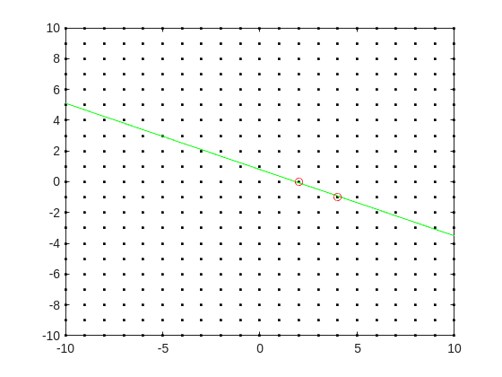
Now, some might think in terms of orthogonal distance to the line, but really, we want the vertical distance to be minimized. Again, minimize abs(delta) in the equation:
log2(3.6) + delta = p + log2(5)*q
where p and q are integer.
Can we do that using MATLAB? The skill about about mathematics often lies in formulating a word problem, and then turning the word problem into a problem of mathematics that we know how to solve. We are almost there now. I next want to formulate this into a problem that intlinprog can solve. The problem at first is intlinprog cannot handle absolute value constraints. And the trick there is to employ slack variables, a terribly useful tool to emply on this class of problem.
Rewrite delta as:
delta = Dpos - Dneg
where Dpos and Dneg are real variables, but both are constrained to be positive.
prob = optimproblem;
p = optimvar('p',lower = -50,upper = 50,type = 'integer');
q = optimvar('q',lower = -50,upper = 50,type = 'integer');
Dpos = optimvar('Dpos',lower = 0);
Dneg = optimvar('Dneg',lower = 0);
Our goal for the ILP solver will be to minimize Dpos + Dneg now. But since they must both be positive, it solves the min absolute value objective. One of them will always be zero.
r = 3.6;
prob.Constraints = log2(r) + Dpos - Dneg == p + log2(5)*q;
prob.Objective = Dpos + Dneg;
The solve is now a simple one. I'll tell it to use intlinprog, even though it would probably figure that out by itself. (Note: if I do not tell solve which solver to use, it does use intlinprog. But it also finds the correct solution when I told it to use GA offline.)
solve(prob,solver = 'intlinprog')
The solution it finds within the bounds of +/- 50 for both p and q seems pretty good. Note that Dpos and Dneg are pretty close to zero.
2^39*5^-16
and while 3.6028979... seems like nothing special, in fact, it is of the form we want.
R = sym(2)^39*sym(5)^-16
vpa(R,100)
vpa(1/R,100)
both of those numbers are exact. If I wanted to find a better approximation to 3.6, all I need do is extend the bounds on p and q. And we can use the same solution approch for any floating point number.
Do you have a swag signed by Brian Douglas? He does!
I came across this fun video from @Christoper Lum, and I have to admit—his MathWorks swag collection is pretty impressive! He’s got pieces I even don’t have.
So now I’m curious… what MathWorks swag do you have hiding in your office or closet?
- Which one is your favorite?
- Which ones do you want to add to your collection?
Show off your swag and share it with the community! 🚀
Since R2024b, a Levenberg–Marquardt solver (TrainingOptionsLM) was introduced. The built‑in function trainnet now accepts training options via the trainingOptions function (https://www.mathworks.com/help/deeplearning/ref/trainingoptions.html#bu59f0q-2) and supports the LM algorithm. I have been curious how to use it in deep learning, and the official documentation has not provided a concrete usage example so far. Below I give a simple example to illustrate how to use this LM algorithm to optimize a small number of learnable parameters.
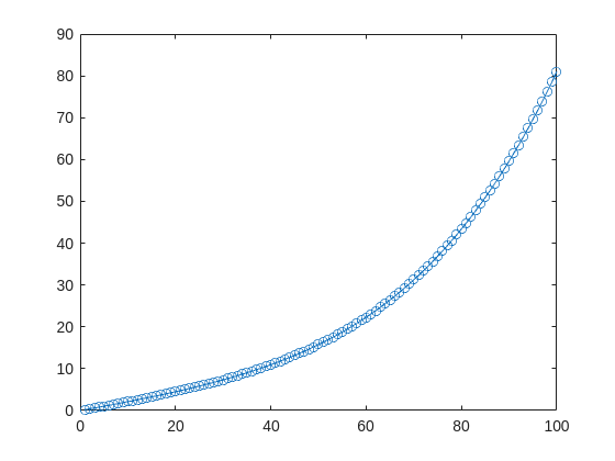
For example, consider the nonlinear function:
y_hat = @(a,t) a(1)*(t/100) + a(2)*(t/100).^2 + a(3)*(t/100).^3 + a(4)*(t/100).^4;
It represents a curve. Given 100 matching points (t → y_hat), we want to use least squares to estimate the four parameters a1–a4.
t = (1:100)';
y_hat = @(a,t)a(1)*(t/100) + a(2)*(t/100).^2 + a(3)*(t/100).^3 + a(4)*(t/100).^4;
x_true = [ 20 ; 10 ; 1 ; 50 ];
y_true = y_hat(x_true,t);
plot(t,y_true,'o-')
- Using the traditional lsqcurvefit-wrapped "Levenberg–Marquardt" algorithm:
x_guess = [ 5 ; 2 ; 0.2 ; -10 ];
options = optimoptions("lsqcurvefit",Algorithm="levenberg-marquardt",MaxFunctionEvaluations=800);
[x,resnorm,residual,exitflag] = lsqcurvefit(y_hat,x_guess,t,y_true,-50*ones(4,1),60*ones(4,1),options);
x,resnorm,exitflag
- Using the deep-learning-wrapped "Levenberg–Marquardt" algorithm:
options = trainingOptions("lm", ...
InitialDampingFactor=0.002, ...
MaxDampingFactor=1e9, ...
DampingIncreaseFactor=12, ...
DampingDecreaseFactor=0.2,...
GradientTolerance=1e-6, ...
StepTolerance=1e-6,...
Plots="training-progress");
numFeatures = 1;
layers = [featureInputLayer(numFeatures,'Name','input')
fitCurveLayer(Name='fitCurve')];
net = dlnetwork(layers);
XData = dlarray(t);
YData = dlarray(y_true);
netTrained = trainnet(XData,YData,net,"mse",options);
netTrained.Layers(2)
classdef fitCurveLayer < nnet.layer.Layer ...
& nnet.layer.Acceleratable
% Example custom SReLU layer.
properties (Learnable)
% Layer learnable parameters
a1
a2
a3
a4
end
methods
function layer = fitCurveLayer(args)
arguments
args.Name = "lm_fit";
end
% Set layer name.
layer.Name = args.Name;
% Set layer description.
layer.Description = "fit curve layer";
end
function layer = initialize(layer,~)
% layer = initialize(layer,layout) initializes the layer
% learnable parameters using the specified input layout.
if isempty(layer.a1)
layer.a1 = rand();
end
if isempty(layer.a2)
layer.a2 = rand();
end
if isempty(layer.a3)
layer.a3 = rand();
end
if isempty(layer.a4)
layer.a4 = rand();
end
end
function Y = predict(layer, X)
% Y = predict(layer, X) forwards the input data X through the
% layer and outputs the result Y.
% Y = layer.a1.*exp(-X./layer.a2) + layer.a3.*X.*exp(-X./layer.a4);
Y = layer.a1*(X/100) + layer.a2*(X/100).^2 + layer.a3*(X/100).^3 + layer.a4*(X/100).^4;
end
end
end
The network is very simple — only the fitCurveLayer defines the learnable parameters a1–a4. I observed that the output values are very close to those from lsqcurvefit.
I saw this YouTube short on my feed: What is MATLab?

I was mostly mesmerized by the minecraft gameplay going on in the background.
Found it funny, thought i'd share.
Trinity
- It's the question that drives us, Neo. It's the question that brought you here. You know the question, just as I did.
Neo
- What is the Matlab?
Morpheus
- Unfortunately, no one can be told what the Matlab is. You have to see it for yourself.
And also later :
Morpheus
- The Matlab is everywhere. It is all around us. Even now, in this very room. You can feel it when you go to work [...]
The Architect
- The first Matlab I designed was quite naturally perfect. It was a work of art. Flawless. Sublime.
[My Matlab quotes version of the movie (Matrix, 1999) ]
Function Syntax Design Conundrum
As a MATLAB enthusiast, I particularly enjoy Steve Eddins' blog and the cool things he explores. MATLAB's new argument blocks are great, but there's one frustrating limitation that Steve outlined beautifully in his blog post "Function Syntax Design Conundrum": cases where an argument should accept both enumerated values AND other data types.
Steve points out this could be done using the input parser, but I prefer having tab completions and I'm not a fan of maintaining function signature JSON files for all my functions.
Personal Context on Enumerations
To be clear: I honestly don't like enumerations in any way, shape, or form. One reason is how awkward they are. I've long suspected they're simply predefined constructor calls with a set argument, and I think that's all but confirmed here. This explains why I've had to fight the enumeration system when trying to take arguments of many types and normalize them to enumerated members, or have numeric values displayed as enumerated members without being recast to the superclass every operation.
The Discovery
While playing around extensively with metadata for another project, I realized (and I'm entirely unsure why it took so long) that the properties of a metaclass object are just, in many cases, the attributes of the classdef. In this realization, I found a solution to Steve's and my problem.
To be clear: I'm not in love with this solution. I would much prefer a better approach for allowing variable sets of membership validation for arguments. But as it stands, we don't have that, so here's an interesting, if incredibly hacky, solution.
If you call struct() on a metaclass object to view its hidden properties, you'll notice that in addition to the public "Enumeration" property, there's a hidden "Enumerable" property. They're both logicals, which implies they're likely functionally distinct. I was curious about that distinction and hoped to find some functionality by intentionally manipulating these values - and I did, solving the exact problem Steve mentions.
The Problem Statement
We have a function with an argument that should allow "dual" input types: enumerated values (Steve's example uses days of the week, mine uses the "all" option available in various dimension-operating functions) AND integers. We want tab completion for the enumerated values while still accepting the numeric inputs.
A Solution for Tab-Completion Supported Arguments
Rather than spoil Steve's blog post, let me use my own example: implementing a none() function. The definition is simple enough tf = ~any(A, dim); but when we wrap this in another function, we lose the tab-completion that any() provides for the dim argument (which gives you "all"). There's no great way to implement this as a function author currently - at least, that's well documented.
So here's my solution:
%% Example Function Implementation
% This is a simple implementation of the DimensionArgument class for implementing dual type inputs that allow enumerated tab-completion.
function tf = none(A, dim)
arguments(Input)
A logical;
dim DimensionArgument = DimensionArgument(A, true);
end
% Simple example (notice the use of uplus to unwrap the hidden property)
tf = ~any(A, +dim);
end
I like this approach because the additional work required to implement it, once the enumeration class is initialized, is minimal. Here are examples of function calls, note that the behavior parallels that of the MATLAB native-style tab-completion:
%% Test Data
% Simple logical array for testing
A = randi([0, 1], [3, 5], "logical");
%% Example function calls
tf = none(A, "all"); % This is the tab-completion it's 1:1 with MATLABs behavior
tf = none(A, [1, 2]); % We can still use valid arguments (validated in the constructor)
tf = none(A); % Showcase of the constructors use as a default argument generator
How It Works
What makes this work is the previously mentioned Enumeration attribute. By setting Enumeration = false while still declaring an enumeration block in the classdef file, we get the suggested members as auto-complete suggestions. As I hinted at, the value of enumerations (if you don't subclass a builtin and define values with the someMember (1) syntax) are simply arguments to constructor calls.
We also get full control over the storage and handling of the class, which means we lose the implicit storage that enumerations normally provide and are responsible for doing so ourselves - but I much prefer this. We can implement internal validation logic to ensure values that aren't in the enumerated set still comply with our constraints, and store the input (whether the enumerated member or alternative type) in an internal property.
As seen in the example class below, this maintains a convenient interface for both the function caller and author the only particuarly verbose portion is the conversion methods... Which if your willing to double down on the uplus unwrapping context can be avoided. What I have personally done is overload the uplus function to return the input (or perform the identity property) this allowss for the uplus to be used universally to unwrap inputs and for those that cant, and dont have a uplus definition, the value itself is just returned:
classdef(Enumeration = false) DimensionArgument % < matlab.mixin.internal.MatrixDisplay
%DimensionArgument Enumeration class to provide auto-complete on functions needing the dimension type seen in all()
% Enumerations are just macros to make constructor calls with a known set of arguments. Declaring the 'all'
% enumeration member means this class can be set as the type for an input and the auto-completion for the given
% argument will show the enumeration members, allowing tab-completion. Declaring the Enumeration attribute of
% the class as false gives us control over the constructor and internal implementation. As such we can use it
% to validate the numeric inputs, in the event the 'all' option was not used, and return an object that will
% then work in place of valid dimension argument options.
%% Enumeration members
% These are the auto-complete options you'd like to make available for the function signature for a given
% argument.
enumeration(Description="Enumerated value for the dimension argument.")
all
end
%% Properties
% The internal property allows the constructor's input to be stored; this ensures that the value is store and
% that the output of the constructor has the class type so that the validation passes.
% (Constructors must return the an object of the class they're a constructor for)
properties(Hidden, Description="Storage of the constructor input for later use.")
Data = [];
end
%% Constructor method
% By the magic of declaring (Enumeration = false) in our class def arguments we get full control over the
% constructor implementation.
%
% The second argument in this specific instance is to enable the argument's default value to be set in the
% arguments block itself as opposed to doing so in the function body... I like this better but if you didn't
% you could just as easily keep the constructor simple.
methods
function obj = DimensionArgument(A, Adim)
%DimensionArgument Initialize the dimension argument.
arguments
% This will be the enumeration member name from auto-completed entries, or the raw user input if not
% used.
A = [];
% A flag that indicates to create the value using different logic, in this case the first non-singleton
% dimension, because this matches the behavior of functions like, all(), sum() prod(), etc.
Adim (1, 1) logical = false;
end
if(Adim)
% Allows default initialization from an input to match the aforemention function's behavior
obj.Data = firstNonscalarDim(A);
else
% As a convenience for this style of implementation we can validate the input to ensure that since we're
% suppose to be an enumeration, the input is valid
DimensionArgument.mustBeValidMember(A);
% Store the input in a hidden property since declaring ~Enumeration means we are responsible for storing
% it.
obj.Data = A;
end
end
end
%% Conversion methods
% Applies conversion to the data property so that implicit casting of functions works. Unfortunately most of
% the MathWorks defined functions use a different system than that employed by the arguments block, which
% defers to the class defined converter methods... Which is why uplus (+obj) has been defined to unwrap the
% data for ease of use.
methods
function obj = uplus(obj)
obj = obj.Data;
end
function str = char(obj)
str = char(obj.Data);
end
function str = cellstr(obj)
str = cellstr(obj.Data);
end
function str = string(obj)
str = string(obj.Data);
end
function A = double(obj)
A = double(obj.Data);
end
function A = int8(obj)
A = int8(obj.Data);
end
function A = int16(obj)
A = int16(obj.Data);
end
function A = int32(obj)
A = int32(obj.Data);
end
function A = int64(obj)
A = int64(obj.Data);
end
end
%% Validation methods
% These utility methods are for input validation
methods(Static, Access = private)
function tf = isValidMember(obj)
%isValidMember Checks that the input is a valid dimension argument.
tf = (istext(obj) && all(obj == "all", "all")) || (isnumeric(obj) && all(isint(obj) & obj > 0, "all"));
end
function mustBeValidMember(obj)
%mustBeValidMember Validates that the input is a valid dimension argument for the dim/dimVec arguments.
if(~DimensionArgument.isValidMember(obj))
exception("JB:DimensionArgument:InvalidInput", "Input must be an integer value or the term 'all'.")
end
end
end
%% Convenient data display passthrough
methods
function disp(obj, name)
arguments
obj DimensionArgument
name string {mustBeScalarOrEmpty} = [];
end
% Dispatch internal data's display implementation
display(obj.Data, char(name));
end
end
end
In the event you'd actually play with theres here are the function definitions for some of the utility functions I used in them, including my exception would be a pain so i wont, these cases wont use it any...
% Far from my definition isint() but is consistent with mustBeInteger() for real numbers but will suffice for the example
function tf = isint(A)
arguments
A {mustBeNumeric(A)};
end
tf = floor(A) == A
end
% Sort of the same but its fine
function dim = firstNonscalarDim(A)
arguments
A
end
dim = [find(size(A) > 1, 1), 0];
dim(1) = dim(1);
end
Hello MATLAB Central, this is my first article.
My name is Yann. And I love MATLAB.
I also love HTTP (i know, weird fetish)
So i started a conversation with ChatGPT about it:
gitclone('https://github.com/yanndebray/HTTP-with-MATLAB');
cd('HTTP-with-MATLAB')
http_with_MATLAB
I'm not sure that this platform is intended to clone repos from github, but i figured I'd paste this shortcut in case you want to try out my live script http_with_MATLAB.m
A lot of what i program lately relies on external web services (either for fetching data, or calling LLMs).
So I wrote a small tutorial of the 7 or so things I feel like I need to remember when making HTTP requests in MATLAB.
Let me know what you think
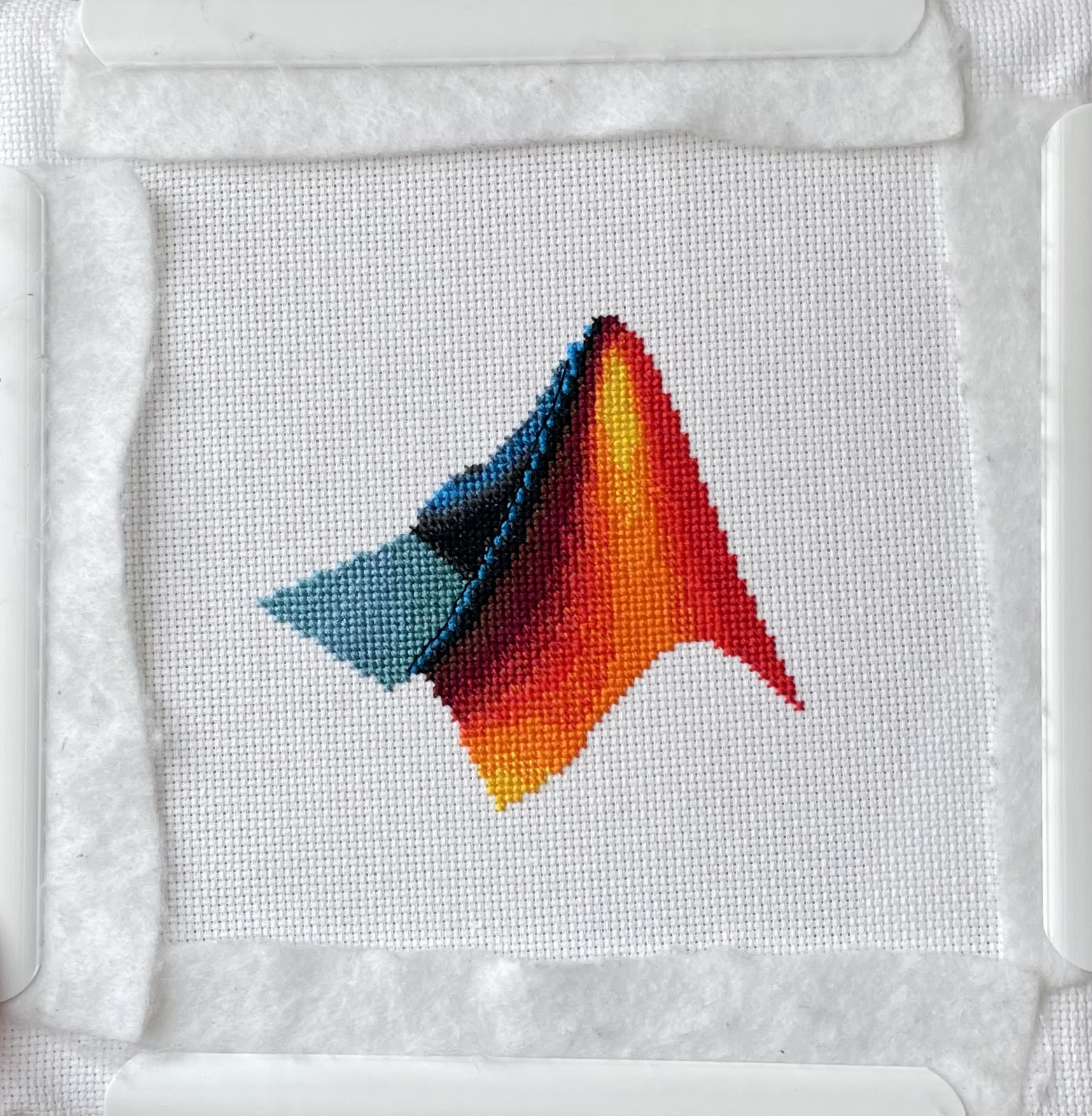
I designed and stitched this last week! It uses a total of 20 DMC thread colors, and I frequently stitched with two colors at once to create the gradient.
Did you know that function double with string vector input significantly outperforms str2double with the same input:
x = rand(1,50000);
t = string(x);
tic; str2double(t); toc
tic; I1 = str2double(t); toc
tic; I2 = double(t); toc
isequal(I1,I2)
Recently I needed to parse numbers from text. I automatically tried to use str2double. However, profiling revealed that str2double was the main bottleneck in my code. Than I realized that there is a new note (since R2024a) in the documentation of str2double:
"Calling string and then double is recommended over str2double because it provides greater flexibility and allows vectorization. For additional information, see Alternative Functionality."
Resharing a fun short video explaining what MATLAB is. :)
t = turtle(); % Start a turtle
t.forward(100); % Move forward by 100
t.backward(100); % Move backward by 100
t.left(90); % Turn left by 90 degrees
t.right(90); % Tur right by 90 degrees
t.goto(100, 100); % Move to (100, 100)
t.turnto(90); % Turn to 90 degrees, i.e. north
t.speed(1000); % Set turtle speed as 1000 (default: 500)
t.pen_up(); % Pen up. Turtle leaves no trace.
t.pen_down(); % Pen down. Turtle leaves a trace again.
t.color('b'); % Change line color to 'b'
t.begin_fill(FaceColor, EdgeColor, FaceAlpha); % Start filling
t.end_fill(); % End filling
t.change_icon('person.png'); % Change the icon to 'person.png'
t.clear(); % Clear the Axes
classdef turtle < handle
properties (GetAccess = public, SetAccess = private)
x = 0
y = 0
q = 0
end
properties (SetAccess = public)
speed (1, 1) double = 500
end
properties (GetAccess = private)
speed_reg = 100
n_steps = 20
ax
l
ht
im
is_pen_up = false
is_filling = false
fill_color
fill_alpha
end
methods
function obj = turtle()
figure(Name='MATurtle', NumberTitle='off')
obj.ax = axes(box="on");
hold on,
obj.ht = hgtransform();
icon = flipud(imread('turtle.png'));
obj.im = imagesc(obj.ht, icon, ...
XData=[-30, 30], YData=[-30, 30], ...
AlphaData=(255 - double(rgb2gray(icon)))/255);
obj.l = plot(obj.x, obj.y, 'k');
obj.ax.XLim = [-500, 500];
obj.ax.YLim = [-500, 500];
obj.ax.DataAspectRatio = [1, 1, 1];
obj.ax.Toolbar.Visible = 'off';
disableDefaultInteractivity(obj.ax);
end
function home(obj)
obj.x = 0;
obj.y = 0;
obj.ht.Matrix = eye(4);
end
function forward(obj, dist)
obj.step(dist);
end
function backward(obj, dist)
obj.step(-dist)
end
function step(obj, delta)
if numel(delta) == 1
delta = delta*[cosd(obj.q), sind(obj.q)];
end
if obj.is_filling
obj.fill(delta);
else
obj.move(delta);
end
end
function goto(obj, x, y)
dx = x - obj.x;
dy = y - obj.y;
obj.turnto(rad2deg(atan2(dy, dx)));
obj.step([dx, dy]);
end
function left(obj, q)
obj.turn(q);
end
function right(obj, q)
obj.turn(-q);
end
function turnto(obj, q)
obj.turn(obj.wrap_angle(q - obj.q, -180));
end
function pen_up(obj)
if obj.is_filling
warning('not available while filling')
return
end
obj.is_pen_up = true;
end
function pen_down(obj, go)
if obj.is_pen_up
if nargin == 1
obj.l(end+1) = plot(obj.x, obj.y, Color=obj.l(end).Color);
else
obj.l(end+1) = go;
end
uistack(obj.ht, 'top')
end
obj.is_pen_up = false;
end
function color(obj, line_color)
if obj.is_filling
warning('not available while filling')
return
end
obj.pen_up();
obj.pen_down(plot(obj.x, obj.y, Color=line_color));
end
function begin_fill(obj, FaceColor, EdgeColor, FaceAlpha)
arguments
obj
FaceColor = [.6, .9, .6];
EdgeColor = [0 0.4470 0.7410];
FaceAlpha = 1;
end
if obj.is_filling
warning('already filling')
return
end
obj.fill_color = FaceColor;
obj.fill_alpha = FaceAlpha;
obj.pen_up();
obj.pen_down(patch(obj.x, obj.y, [1, 1, 1], ...
EdgeColor=EdgeColor, FaceAlpha=0));
obj.is_filling = true;
end
function end_fill(obj)
if ~obj.is_filling
warning('not filling now')
return
end
obj.l(end).FaceColor = obj.fill_color;
obj.l(end).FaceAlpha = obj.fill_alpha;
obj.is_filling = false;
end
function change_icon(obj, filename)
icon = flipud(imread(filename));
obj.im.CData = icon;
obj.im.AlphaData = (255 - double(rgb2gray(icon)))/255;
end
function clear(obj)
obj.x = 0;
obj.y = 0;
delete(obj.ax.Children(2:end));
obj.l = plot(0, 0, 'k');
obj.ht.Matrix = eye(4);
end
end
methods (Access = private)
function animated_step(obj, delta, q, initFcn, updateFcn)
arguments
obj
delta
q
initFcn = @() []
updateFcn = @(~, ~) []
end
dx = delta(1)/obj.n_steps;
dy = delta(2)/obj.n_steps;
dq = q/obj.n_steps;
pause_duration = norm(delta)/obj.speed/obj.speed_reg;
initFcn();
for i = 1:obj.n_steps
updateFcn(dx, dy);
obj.ht.Matrix = makehgtform(...
translate=[obj.x + dx*i, obj.y + dy*i, 0], ...
zrotate=deg2rad(obj.q + dq*i));
pause(pause_duration)
drawnow limitrate
end
obj.x = obj.x + delta(1);
obj.y = obj.y + delta(2);
end
function obj = turn(obj, q)
obj.animated_step([0, 0], q);
obj.q = obj.wrap_angle(obj.q + q, 0);
end
function move(obj, delta)
initFcn = @() [];
updateFcn = @(dx, dy) [];
if ~obj.is_pen_up
initFcn = @() initializeLine();
updateFcn = @(dx, dy) obj.update_end_point(obj.l(end), dx, dy);
end
function initializeLine()
obj.l(end).XData(end+1) = obj.l(end).XData(end);
obj.l(end).YData(end+1) = obj.l(end).YData(end);
end
obj.animated_step(delta, 0, initFcn, updateFcn);
end
function obj = fill(obj, delta)
initFcn = @() initializePatch();
updateFcn = @(dx, dy) obj.update_end_point(obj.l(end), dx, dy);
function initializePatch()
obj.l(end).Vertices(end+1, :) = obj.l(end).Vertices(end, :);
obj.l(end).Faces = 1:size(obj.l(end).Vertices, 1);
end
obj.animated_step(delta, 0, initFcn, updateFcn);
end
end
methods (Static, Access = private)
function update_end_point(l, dx, dy)
l.XData(end) = l.XData(end) + dx;
l.YData(end) = l.YData(end) + dy;
end
function q = wrap_angle(q, min_angle)
q = mod(q - min_angle, 360) + min_angle;
end
end
end
I would like to zoom directly on the selected region when using  on my image created with image or imagesc. First of all, I would recommend using image or imagesc and not imshow for this case, see comparison here: Differences between imshow() and image()? However when zooming Stretch-to-Fill behavior happens and I don't want that. Try range zoom to image generated by this code:
fig = uifigure;
ax = uiaxes(fig);
im = imread("peppers.png");
h = imagesc(im,"Parent",ax);
axis(ax,'tight', 'off')
I can fix that with manualy setting data aspect ratio:
daspect(ax,[1 1 1])
However, I need this code to run automatically after zooming. So I create zoom object and ActionPostCallback which is called everytime after I zoom, see zoom - ActionPostCallback.
z = zoom(ax);
z.ActionPostCallback = @(fig,ax) daspect(ax.Axes,[1 1 1]);
If you need, you can also create ActionPreCallback which is called everytime before I zoom, see zoom - ActionPreCallback.
z.ActionPreCallback = @(fig,ax) daspect(ax.Axes,'auto');
Code written and run in R2025a.
I am thrilled python interoperability now seems to work for me with my APPLE M1 MacBookPro and MATLAB V2025a. The available instructions are still, shall we say, cryptic. Here is a summary of my interaction with GPT 4o to get this to work.
===========================================================
MATLAB R2025a + Python (Astropy) Integration on Apple Silicon (M1/M2/M3 Macs)
===========================================================
Author: D. Carlsmith, documented with ChatGPT
Last updated: July 2025
This guide provides full instructions, gotchas, and workarounds to run Python 3.10 with MATLAB R2025a (Apple Silicon/macOS) using native ARM64 Python and calling modules like Astropy, Numpy, etc. from within MATLAB.
===========================================================
Overview
===========================================================
- MATLAB R2025a on Apple Silicon (M1/M2/M3) runs as "maca64" (native ARM64).
- To call Python from MATLAB, the Python interpreter must match that architecture (ARM64).
- Using Intel Python (x86_64) with native MATLAB WILL NOT WORK.
- The cleanest solution: use Miniforge3 (Conda-forge's lightweight ARM64 distribution).
===========================================================
1. Install Miniforge3 (ARM64-native Conda)
===========================================================
In Terminal, run:
curl -LO https://github.com/conda-forge/miniforge/releases/latest/download/Miniforge3-MacOSX-arm64.sh
bash Miniforge3-MacOSX-arm64.sh
Follow prompts:
- Press ENTER to scroll through license.
- Type "yes" when asked to accept the license.
- Press ENTER to accept the default install location: ~/miniforge3
- When asked:
Do you wish to update your shell profile to automatically initialize conda? [yes|no]
Type: yes
===========================================================
2. Restart Terminal and Create a Python Environment for MATLAB
===========================================================
Run the following:
conda create -n matlab python=3.10 astropy numpy -y
conda activate matlab
Verify the Python path:
which python
Expected output:
/Users/YOURNAME/miniforge3/envs/matlab/bin/python
===========================================================
3. Verify Python + Astropy From Terminal
===========================================================
Run:
python -c "import astropy; print(astropy.__version__)"
Expected output:
6.x.x (or similar)
===========================================================
4. Configure MATLAB to Use This Python
===========================================================
In MATLAB R2025a (Apple Silicon):
clear classes
pyenv('Version', '/Users/YOURNAME/miniforge3/envs/matlab/bin/python')
py.sys.version
You should see the Python version printed (e.g. 3.10.18). No error means it's working.
===========================================================
5. Gotchas and Their Solutions
===========================================================
❌ Error: Python API functions are not available
→ Cause: Wrong architecture or broken .dylib
→ Fix: Use Miniforge ARM64 Python. DO NOT use Intel Anaconda.
❌ Error: Invalid text character (↑ points at __version__)
→ Cause: MATLAB can’t parse double underscores typed or pasted
→ Fix: Use: py.getattr(module, '__version__')
❌ Error: Unrecognized method 'separation' or 'sec'
→ Cause: MATLAB can't reflect dynamic Python methods
→ Fix: Use: py.getattr(obj, 'method')(args)
===========================================================
6. Run Full Verification in MATLAB
===========================================================
Paste this into MATLAB:
% Set environment
clear classes
pyenv('Version', '/Users/YOURNAME/miniforge3/envs/matlab/bin/python');
% Import modules
coords = py.importlib.import_module('astropy.coordinates');
time_mod = py.importlib.import_module('astropy.time');
table_mod = py.importlib.import_module('astropy.table');
% Astropy version
ver = char(py.getattr(py.importlib.import_module('astropy'), '__version__'));
disp(['Astropy version: ', ver]);
% SkyCoord angular separation
c1 = coords.SkyCoord('10h21m00s', '+41d12m00s', pyargs('frame', 'icrs'));
c2 = coords.SkyCoord('10h22m00s', '+41d15m00s', pyargs('frame', 'icrs'));
sep_fn = py.getattr(c1, 'separation');
sep = sep_fn(c2);
arcsec = double(sep.to('arcsec').value);
fprintf('Angular separation = %.3f arcsec\n', arcsec);
% Time difference in seconds
Time = time_mod.Time;
t1 = Time('2025-01-01T00:00:00', pyargs('format','isot','scale','utc'));
t2 = Time('2025-01-02T00:00:00', pyargs('format','isot','scale','utc'));
dt = py.getattr(t2, '__sub__')(t1);
seconds = double(py.getattr(dt, 'sec'));
fprintf('Time difference = %.0f seconds\n', seconds);
% Astropy table display
tbl = table_mod.Table(pyargs('names', {'a','b'}, 'dtype', {'int','float'}));
tbl.add_row({1, 2.5});
tbl.add_row({2, 3.7});
disp(tbl);
===========================================================
7. Optional: Automatically Configure Python in startup.m
===========================================================
To avoid calling pyenv() every time, edit your MATLAB startup:
edit startup.m
Add:
try
pyenv('Version', '/Users/YOURNAME/miniforge3/envs/matlab/bin/python');
catch
warning("Python already loaded.");
end
===========================================================
8. Final Notes
===========================================================
- This setup avoids all architecture mismatches.
- It uses a clean, minimal ARM64 Python that integrates seamlessly with MATLAB.
- Do not mix Anaconda (Intel) with Apple Silicon MATLAB.
- Use py.getattr for any Python attribute containing underscores or that MATLAB can't resolve.
You can now run NumPy, Astropy, Pandas, Astroquery, Matplotlib, and more directly from MATLAB.
===========================================================
Hey MATLAB enthusiasts!
I just stumbled upon this hilariously effective GitHub repo for image deformation using Moving Least Squares (MLS)—and it’s pure gold for anyone who loves playing with pixels! 🎨✨
- Real-Time Magic ✨
- Precomputes weights and deformation data upfront, making it blazing fast for interactive edits. Drag control points and watch the image warp like rubber! (2)
- Supports affine, similarity, and rigid deformations—because why settle for one flavor of chaos?
- Single-File Simplicity 🧩
- All packed into one clean MATLAB class (mlsImageWarp.m).
- Endless Fun Use Cases 🤹
- Turn your pet’s photo into a Picasso painting.
- "Fix" your friend’s smile... aggressively.
- Animate static images with silly deformations (1).
Try the Demo!
You are not a jedi yet !
20%
We not grant u the rank of master !
0%
Ready are u? What knows u of ready?
0%
May the Force be with you !
80%
5 个投票
I saw this on Reddit and thought of the past mini-hack contests. We have a few folks here who can do something similar with MATLAB.