The beautiful and elegant chord diagrams were all created using MATLAB?
Indeed, they were all generated using the chord diagram plotting toolkit that I developed myself:
You can download these toolkits from the provided links.
The reason for writing this article is that many people have started using the chord diagram plotting toolkit that I developed. However, some users are unsure about customizing certain styles. As the developer, I have a good understanding of the implementation principles of the toolkit and can apply it flexibly. This has sparked the idea of challenging myself to create various styles of chord diagrams. Currently, the existing code is quite lengthy. In the future, I may integrate some of this code into the toolkit, enabling users to achieve the effects of many lines of code with just a few lines.
Without further ado, let's see the extent to which this MATLAB toolkit can currently perform.
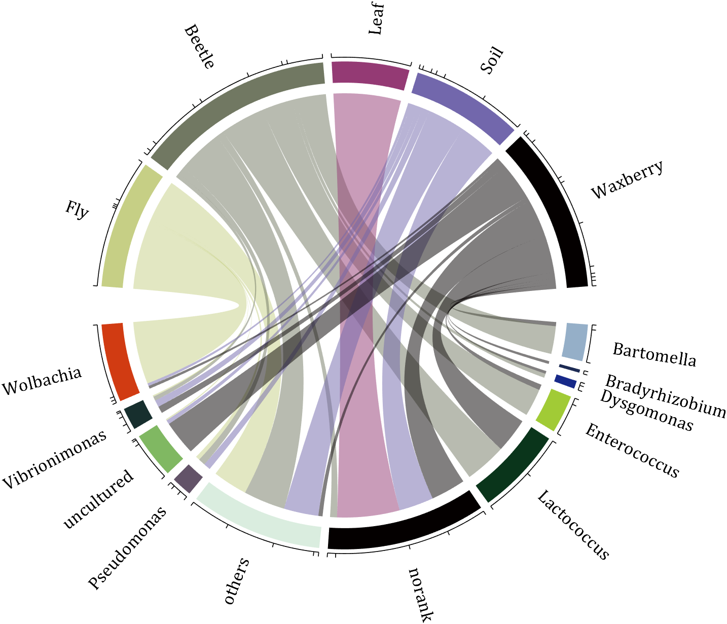
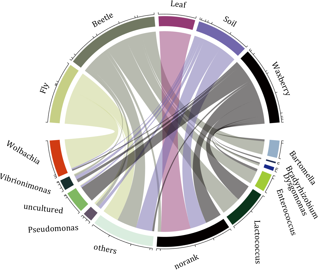
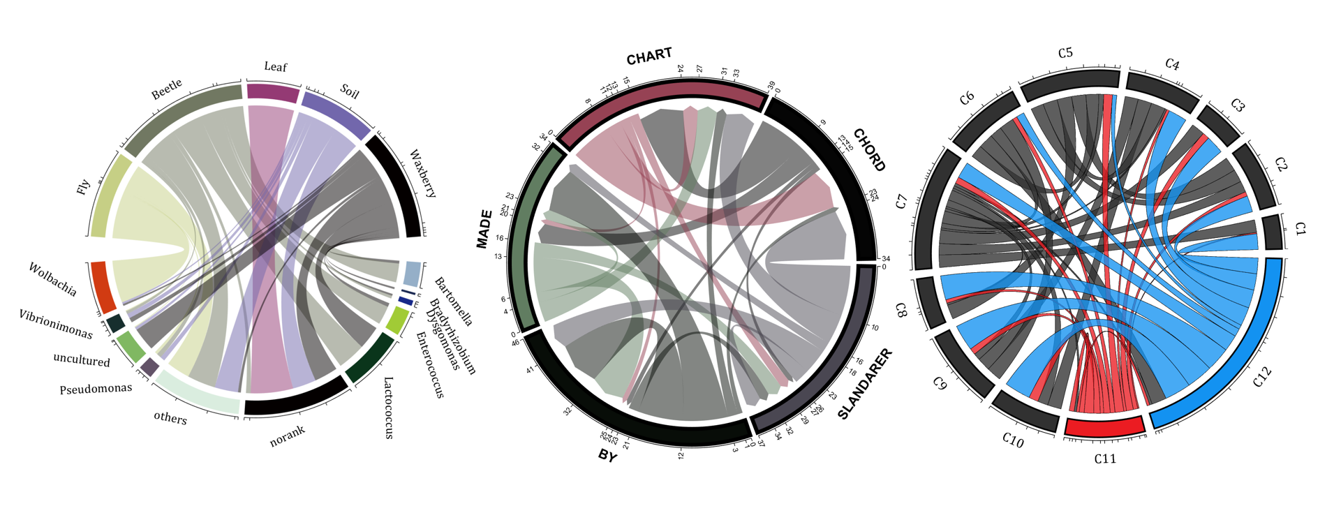
demo 1
rng(2)
dataMat = randi([0,5], [11,5]);
dataMat(1:6,1) = 0;
dataMat([11,7],1) = [45,25];
dataMat([1,4,5,7],2) = [20,20,30,30];
dataMat(:,3) = 0;
dataMat(6,3) = 45;
dataMat(1:5,4) = 0;
dataMat([6,7],4) = [25,25];
dataMat([5,6,9],5) = [25,25,25];
colName = {'Fly', 'Beetle', 'Leaf', 'Soil', 'Waxberry'};
rowName = {'Bartomella', 'Bradyrhizobium', 'Dysgomonas', 'Enterococcus',...
'Lactococcus', 'norank', 'others', 'Pseudomonas', 'uncultured',...
'Vibrionimonas', 'Wolbachia'};
figure('Units','normalized', 'Position',[.02,.05,.6,.85])
CC = chordChart(dataMat, 'rowName',rowName, 'colName',colName, 'Sep',1/80);
CC = CC.draw();
CListT = [0.7765 0.8118 0.5216; 0.4431 0.4706 0.3843; 0.5804 0.2275 0.4549;
0.4471 0.4039 0.6745; 0.0157 0 0 ];
for i = 1:size(dataMat, 2)
CC.setSquareT_N(i, 'FaceColor',CListT(i,:))
end
CListF = [0.5843 0.6863 0.7843; 0.1098 0.1647 0.3255; 0.0902 0.1608 0.5373;
0.6314 0.7961 0.2118; 0.0392 0.2078 0.1059; 0.0157 0 0 ;
0.8549 0.9294 0.8745; 0.3882 0.3255 0.4078; 0.5020 0.7216 0.3843;
0.0902 0.1843 0.1804; 0.8196 0.2314 0.0706];
for i = 1:size(dataMat, 1)
CC.setSquareF_N(i, 'FaceColor',CListF(i,:))
end
for i = 1:size(dataMat, 1)
for j = 1:size(dataMat, 2)
CC.setChordMN(i,j, 'FaceColor',CListT(j,:), 'FaceAlpha',.5)
end
end
CC.tickState('on')
CC.labelRotate('on')
CC.setFont('FontSize',17, 'FontName','Cambria')
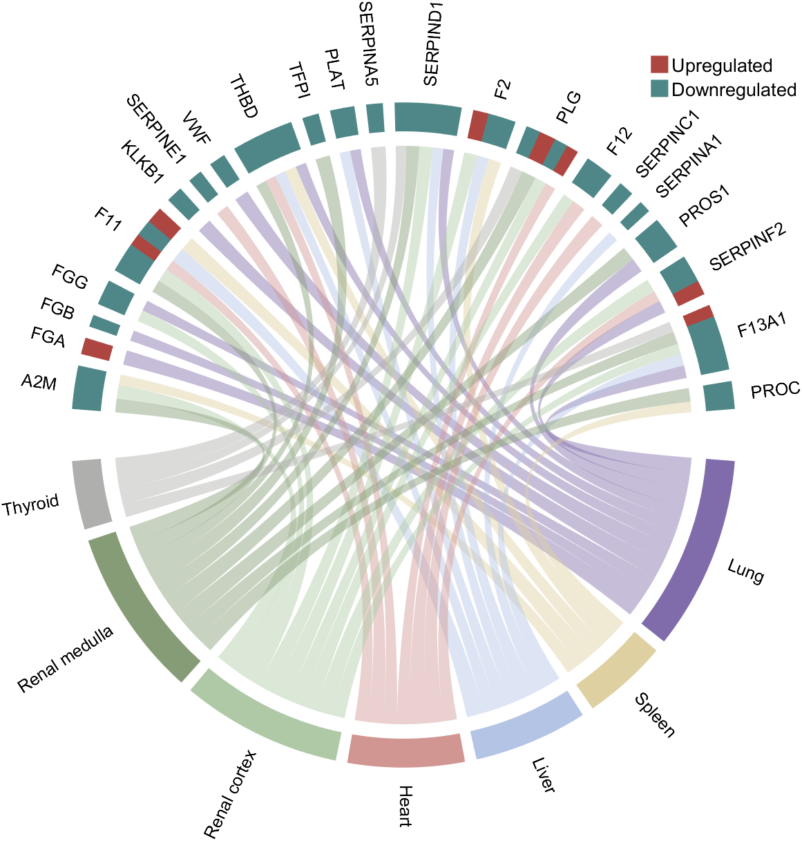
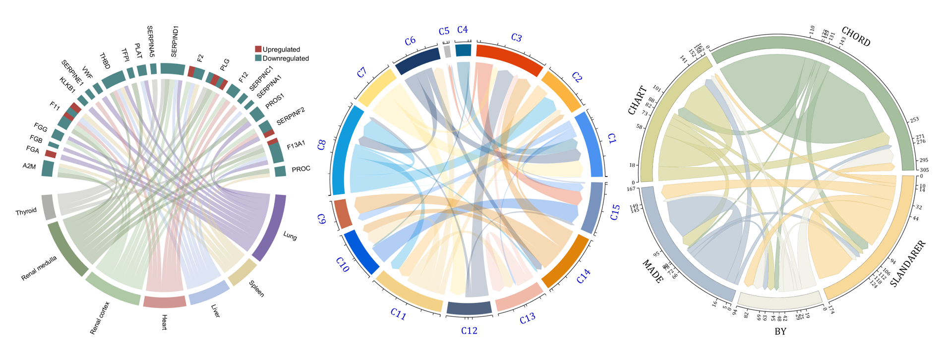
demo 2
rng(3)
dataMat = randi([1,15], [7,22]);
dataMat(dataMat < 11) = 0;
dataMat(1, sum(dataMat, 1) == 0) = 15;
colName = {'A2M', 'FGA', 'FGB', 'FGG', 'F11', 'KLKB1', 'SERPINE1', 'VWF',...
'THBD', 'TFPI', 'PLAT', 'SERPINA5', 'SERPIND1', 'F2', 'PLG', 'F12',...
'SERPINC1', 'SERPINA1', 'PROS1', 'SERPINF2', 'F13A1', 'PROC'};
rowName = {'Lung', 'Spleen', 'Liver', 'Heart',...
'Renal cortex', 'Renal medulla', 'Thyroid'};
figure('Units','normalized', 'Position',[.02,.05,.6,.85])
CC = chordChart(dataMat, 'rowName',rowName, 'colName',colName, 'Sep',1/80, 'LRadius',1.21);
CC = CC.draw();
CC.labelRotate('on')
CListT = [173,70,65; 79,135,136]./255;
Regulated = rand([7, 22]);
Regulated = (Regulated < .8) + 1;
for i = 1:size(Regulated, 1)
for j = 1:size(Regulated, 2)
CC.setEachSquareT_Prop(i, j, 'FaceColor', CListT(Regulated(i,j),:))
end
end
H1 = fill([0,1,0] + 100, [1,0,1] + 100, CListT(1,:), 'EdgeColor','none');
H2 = fill([0,1,0] + 100, [1,0,1] + 100, CListT(2,:), 'EdgeColor','none');
lgdHdl = legend([H1,H2], {'Upregulated','Downregulated'}, 'AutoUpdate','off', 'Location','best');
lgdHdl.ItemTokenSize = [12,12];
lgdHdl.Box = 'off';
lgdHdl.FontSize = 13;
CListF = [128,108,171; 222,208,161; 180,196,229; 209,150,146; 175,201,166;
134,156,118; 175,175,173]./255;
for i = 1:size(dataMat, 1)
CC.setSquareF_N(i, 'FaceColor',CListF(i,:))
end
for i = 1:size(dataMat, 1)
for j = 1:size(dataMat, 2)
CC.setChordMN(i,j, 'FaceColor',CListF(i,:), 'FaceAlpha',.45)
end
end
demo 3
dataMat = rand([15,15]);
dataMat(dataMat > .15) = 0;
CList = [ 75,146,241; 252,180, 65; 224, 64, 10; 5,100,146; 191,191,191;
26, 59,105; 255,227,130; 18,156,221; 202,107, 75; 0, 92,219;
243,210,136; 80, 99,129; 241,185,168; 224,131, 10; 120,147,190]./255;
figure('Units','normalized', 'Position',[.02,.05,.6,.85])
BCC = biChordChart(dataMat, 'Arrow','on', 'CData',CList);
BCC = BCC.draw();
BCC.tickState('on')
BCC.setFont('FontName','Cambria', 'FontSize',17, 'Color',[0,0,.8])
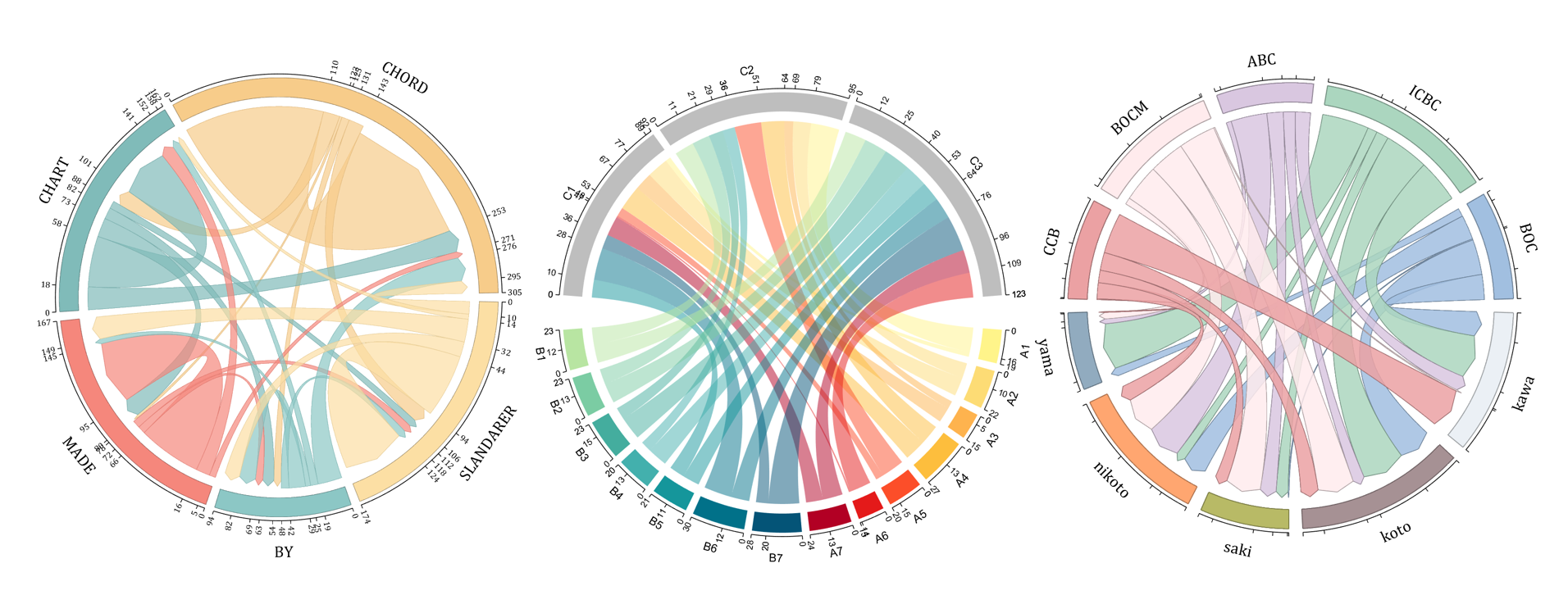
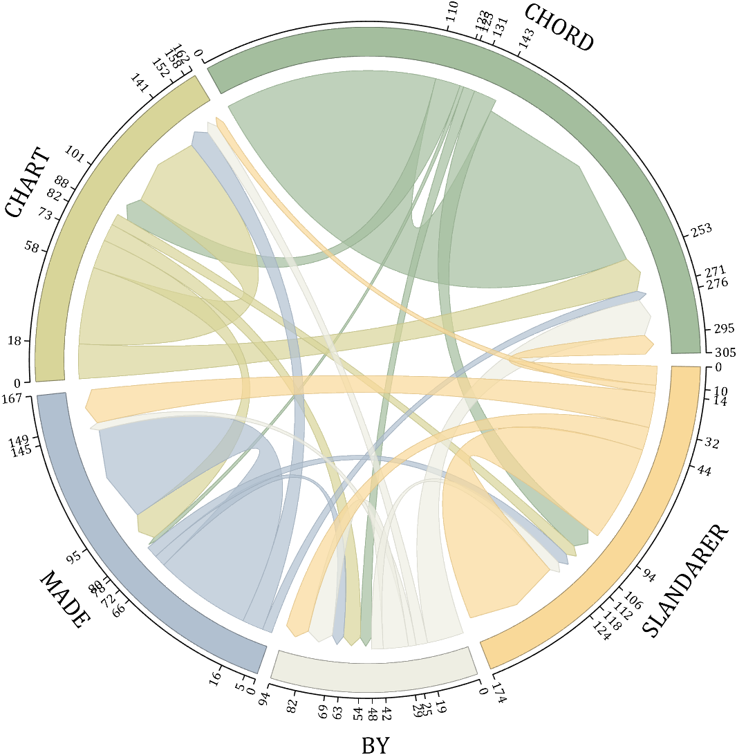
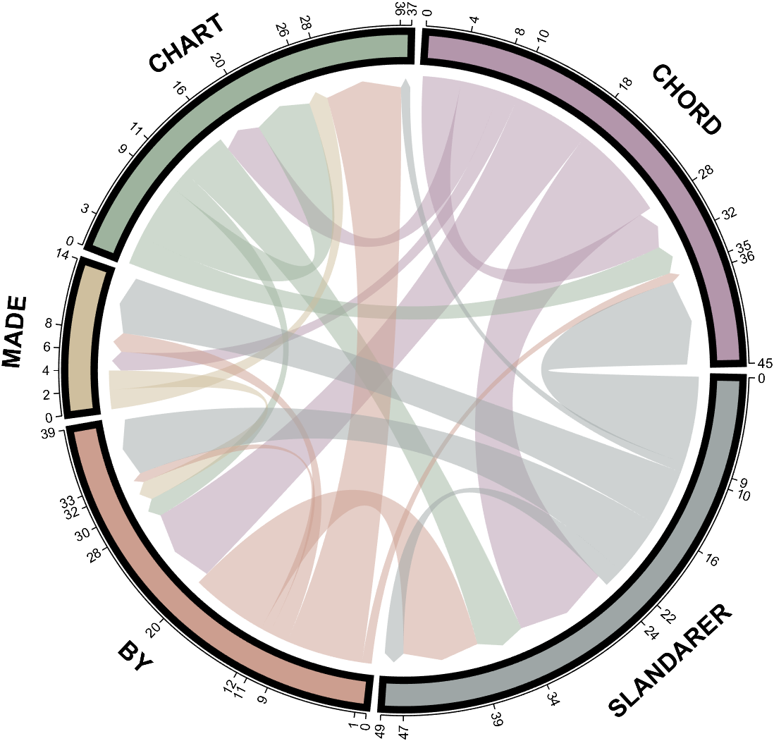
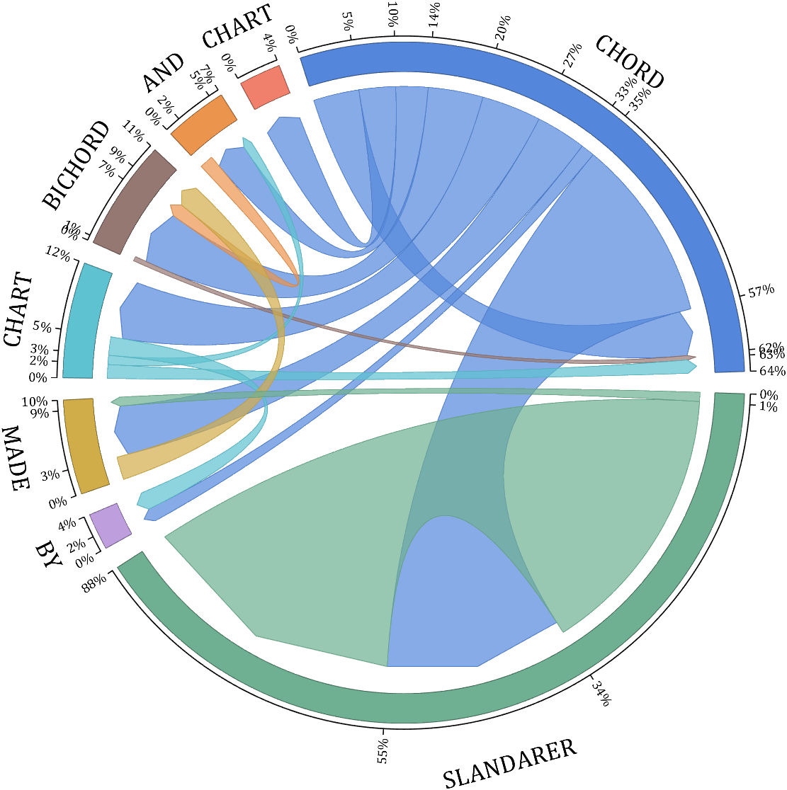
demo 4
rng(5)
dataMat = randi([1,20], [5,5]);
dataMat(1,1) = 110;
dataMat(2,2) = 40;
dataMat(3,3) = 50;
dataMat(5,5) = 50;
CList1 = [164,190,158; 216,213,153; 177,192,208; 238,238,227; 249,217,153]./255;
CList2 = [247,204,138; 128,187,185; 245,135,124; 140,199,197; 252,223,164]./255;
CList = CList2;
NameList={'CHORD','CHART','MADE','BY','SLANDARER'};
figure('Units','normalized', 'Position',[.02,.05,.6,.85])
BCC = biChordChart(dataMat, 'Arrow','on', 'CData',CList, 'Sep',1/30, 'Label',NameList, 'LRadius',1.33);
BCC = BCC.draw();
BCC.tickState('on')
for i = 1:size(dataMat, 1)
for j = 1:size(dataMat, 2)
if dataMat(i,j) > 0
BCC.setChordMN(i,j, 'FaceAlpha',.7, 'EdgeColor',CList(i,:)./1.1)
end
end
end
for i = 1:size(dataMat, 1)
BCC.setSquareN(i, 'EdgeColor',CList(i,:)./1.7)
end
BCC.setFont('FontName','Cambria', 'FontSize',17)
BCC.tickLabelState('on')
BCC.setTickFont('FontName','Cambria', 'FontSize',9)
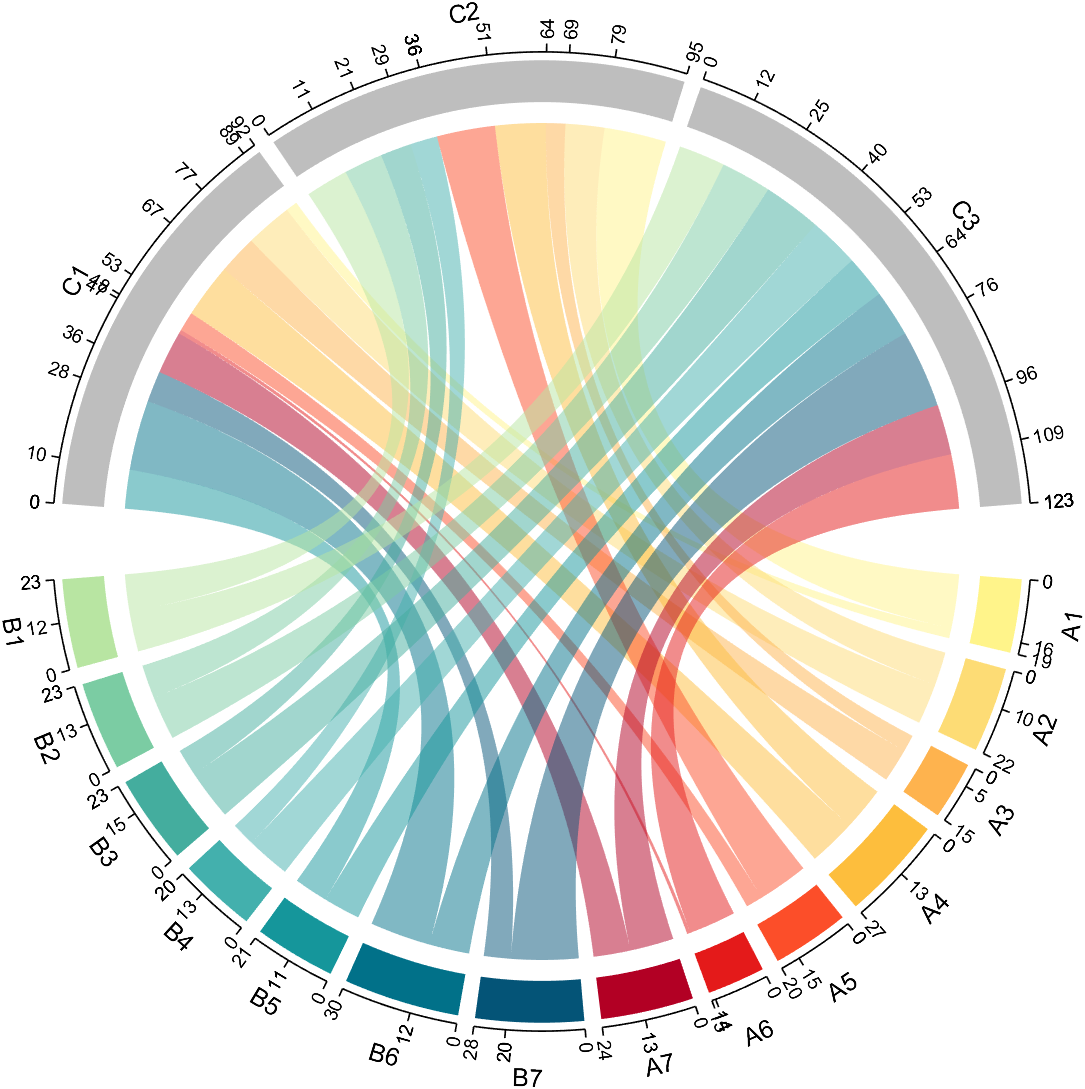
demo 5
dataMat=randi([1,20], [14,3]);
dataMat(11:14,1) = 0;
dataMat(6:10,2) = 0;
dataMat(1:5,3) = 0;
colName = compose('C%d', 1:3);
rowName = [compose('A%d', 1:7), compose('B%d', 7:-1:1)];
figure('Units','normalized', 'Position',[.02,.05,.6,.85])
CC = chordChart(dataMat, 'rowName',rowName, 'colName',colName, 'Sep',1/80);
CC = CC.draw();
for i = 1:size(dataMat, 2)
CC.setSquareT_N(i, 'FaceColor',[190,190,190]./255)
end
CListF=[255,244,138; 253,220,117; 254,179, 78; 253,190, 61;
252, 78, 41; 228, 26, 26; 178, 0, 36; 4, 84,119;
1,113,137; 21,150,155; 67,176,173; 68,173,158;
123,204,163; 184,229,162]./255;
for i = 1:size(dataMat, 1)
CC.setSquareF_N(i, 'FaceColor',CListF(i,:))
end
for i = 1:size(dataMat, 1)
for j = 1:size(dataMat, 2)
CC.setChordMN(i,j, 'FaceColor',CListF(i,:), 'FaceAlpha',.5)
end
end
CC.tickState('on')
CC.tickLabelState('on')
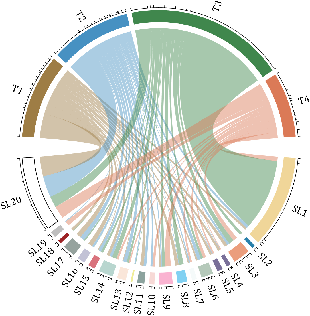
demo 6
rng(2)
dataMat = randi([0,40], [20,4]);
dataMat(rand([20,4]) < .2) = 0;
dataMat(1,3) = 500;
dataMat(20,1:4) = [140; 150; 80; 90];
colName = compose('T%d', 1:4);
rowName = compose('SL%d', 1:20);
figure('Units','normalized', 'Position',[.02,.05,.6,.85])
CC = chordChart(dataMat, 'rowName',rowName, 'colName',colName, 'Sep',1/80, 'LRadius',1.23);
CC = CC.draw();
CListT = [0.62,0.49,0.27; 0.28,0.57,0.76
0.25,0.53,0.30; 0.86,0.48,0.34];
for i = 1:size(dataMat, 2)
CC.setSquareT_N(i, 'FaceColor',CListT(i,:))
end
CListF = [0.94,0.84,0.60; 0.16,0.50,0.67; 0.92,0.62,0.49;
0.48,0.44,0.60; 0.48,0.44,0.60; 0.71,0.79,0.73;
0.96,0.98,0.98; 0.51,0.82,0.95; 0.98,0.70,0.82;
0.97,0.85,0.84; 0.55,0.64,0.62; 0.94,0.93,0.60;
0.98,0.90,0.85; 0.72,0.84,0.81; 0.85,0.45,0.49;
0.76,0.76,0.84; 0.59,0.64,0.62; 0.62,0.14,0.15;
0.75,0.75,0.75; 1.00,1.00,1.00];
for i = 1:size(dataMat, 1)
CC.setSquareF_N(i, 'FaceColor',CListF(i,:))
end
CC.setSquareF_N(size(dataMat, 1), 'EdgeColor','k', 'LineWidth',1)
for i = 1:size(dataMat, 1)
for j = 1:size(dataMat, 2)
CC.setChordMN(i,j, 'FaceColor',CListT(j,:), 'FaceAlpha',.46)
end
end
CC.tickState('on')
CC.labelRotate('on')
CC.setFont('FontSize',17, 'FontName','Cambria')
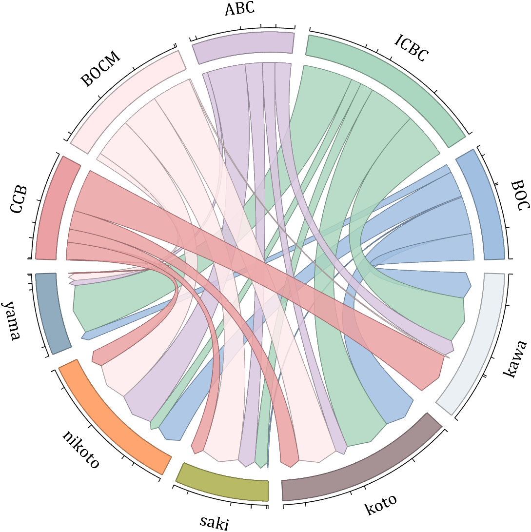
demo 7
dataMat = randi([10,10000], [10,10]);
dataMat(6:10,:) = 0;
dataMat(:,1:5) = 0;
NameList = {'BOC', 'ICBC', 'ABC', 'BOCM', 'CCB', ...
'yama', 'nikoto', 'saki', 'koto', 'kawa'};
CList = [0.63,0.75,0.88
0.67,0.84,0.75
0.85,0.78,0.88
1.00,0.92,0.93
0.92,0.63,0.64
0.57,0.67,0.75
1.00,0.65,0.44
0.72,0.73,0.40
0.65,0.57,0.58
0.92,0.94,0.96];
figure('Units','normalized', 'Position',[.02,.05,.6,.85])
BCC = biChordChart(dataMat, 'Arrow','on', 'CData',CList, 'Label',NameList);
BCC = BCC.draw();
for i = 1:size(dataMat, 1)
for j = 1:size(dataMat, 2)
if dataMat(i,j) > 0
BCC.setChordMN(i,j, 'FaceAlpha',.85, 'EdgeColor',CList(i,:)./1.5, 'LineWidth',.8)
end
end
end
for i = 1:size(dataMat, 1)
BCC.setSquareN(i, 'EdgeColor',CList(i,:)./1.5, 'LineWidth',1)
end
BCC.tickState('on')
BCC.setFont('FontName','Cambria', 'FontSize',17)
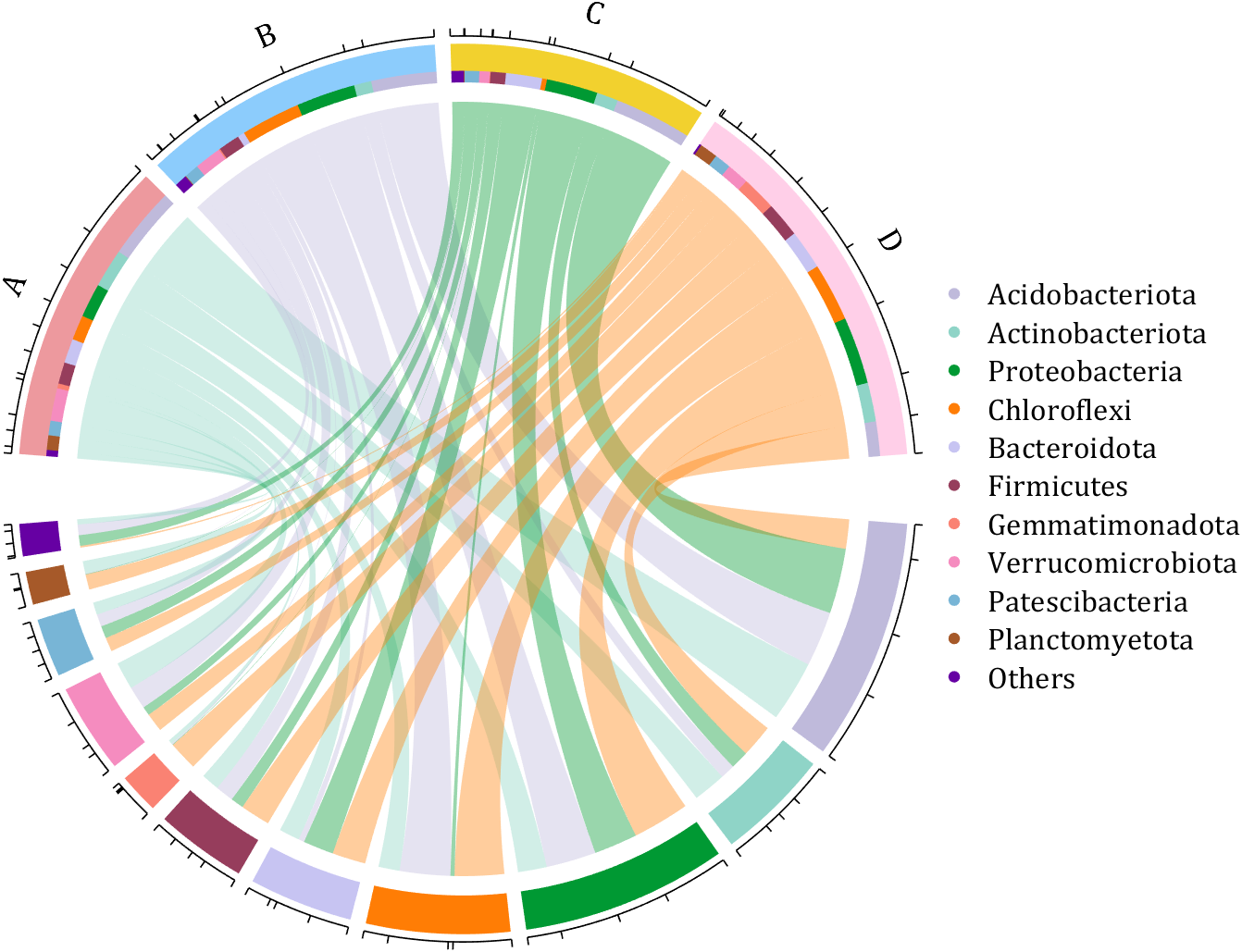
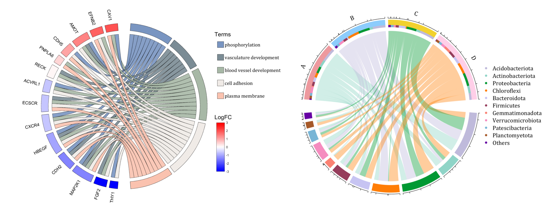
demo 8
dataMat = rand([11,4]);
dataMat = round(10.*dataMat.*((11:-1:1).'+1))./10;
colName = {'A','B','C','D'};
rowName = {'Acidobacteriota', 'Actinobacteriota', 'Proteobacteria', ...
'Chloroflexi', 'Bacteroidota', 'Firmicutes', 'Gemmatimonadota', ...
'Verrucomicrobiota', 'Patescibacteria', 'Planctomyetota', 'Others'};
figure('Units','normalized', 'Position',[.02,.05,.8,.85])
CC = chordChart(dataMat, 'colName',colName, 'Sep',1/80, 'SSqRatio',30/100);
CC = CC.draw();
CListT = [0.93,0.60,0.62
0.55,0.80,0.99
0.95,0.82,0.18
1.00,0.81,0.91];
for i = 1:size(dataMat, 2)
CC.setSquareT_N(i, 'FaceColor',CListT(i,:))
end
CListF = [0.75,0.73,0.86
0.56,0.83,0.78
0.00,0.60,0.20
1.00,0.49,0.02
0.78,0.77,0.95
0.59,0.24,0.36
0.98,0.51,0.45
0.96,0.55,0.75
0.47,0.71,0.84
0.65,0.35,0.16
0.40,0.00,0.64];
for i = 1:size(dataMat, 1)
CC.setSquareF_N(i, 'FaceColor',CListF(i,:))
end
CListC = [0.55,0.83,0.76
0.75,0.73,0.86
0.00,0.60,0.19
1.00,0.51,0.04];
for i = 1:size(dataMat, 1)
for j = 1:size(dataMat, 2)
CC.setChordMN(i,j, 'FaceColor',CListC(j,:), 'FaceAlpha',.4)
end
end
for i = 1:size(dataMat, 1)
for j = 1:size(dataMat, 2)
CC.setEachSquareT_Prop(i,j, 'FaceColor', CListF(i,:))
end
end
CC.tickState('on')
CC.setFont('FontName','Cambria', 'FontSize',17)
textHdl = findobj(gca, 'Tag','ChordLabel');
for i = 1:length(textHdl)
if textHdl(i).Position(2) < 0
set(textHdl(i), 'Visible','off')
end
end
scatterHdl = scatter(10.*ones(size(dataMat,1)),10.*ones(size(dataMat,1)), ...
55, 'filled');
for i = 1:length(scatterHdl)
scatterHdl(i).CData = CListF(i,:);
end
lgdHdl = legend(scatterHdl, rowName, 'Location','best', 'FontSize',16, 'FontName','Cambria', 'Box','off');
set(lgdHdl, 'Position',[.7482,.3577,.1658,.3254])
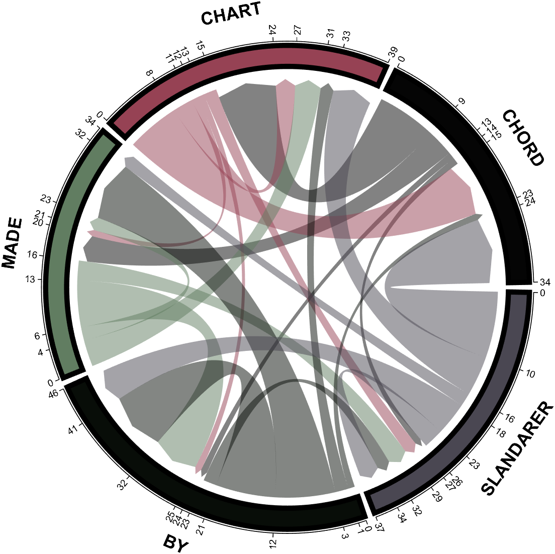
demo 9
dataMat = randi([0,10], [5,5]);
CList1 = [0.70,0.59,0.67
0.62,0.70,0.62
0.81,0.75,0.62
0.80,0.62,0.56
0.62,0.65,0.65];
CList2 = [0.02,0.02,0.02
0.59,0.26,0.33
0.38,0.49,0.38
0.03,0.05,0.03
0.29,0.28,0.32];
CList = CList2;
NameList={'CHORD','CHART','MADE','BY','SLANDARER'};
figure('Units','normalized', 'Position',[.02,.05,.6,.85])
BCC = biChordChart(dataMat, 'Arrow','on', 'CData',CList, 'Sep',1/30, 'Label',NameList, 'LRadius',1.33);
BCC = BCC.draw();
for i = 1:size(dataMat, 1)
for j = 1:size(dataMat, 2)
BCC.setChordMN(i,j, 'FaceAlpha',.5)
end
end
for i = 1:size(dataMat, 1)
BCC.setSquareN(i, 'EdgeColor',[0,0,0], 'LineWidth',5)
end
BCC.tickState('on')
BCC.setFont('FontSize',17, 'FontWeight','bold')
BCC.tickLabelState('on')
BCC.setTickFont('FontSize',9)
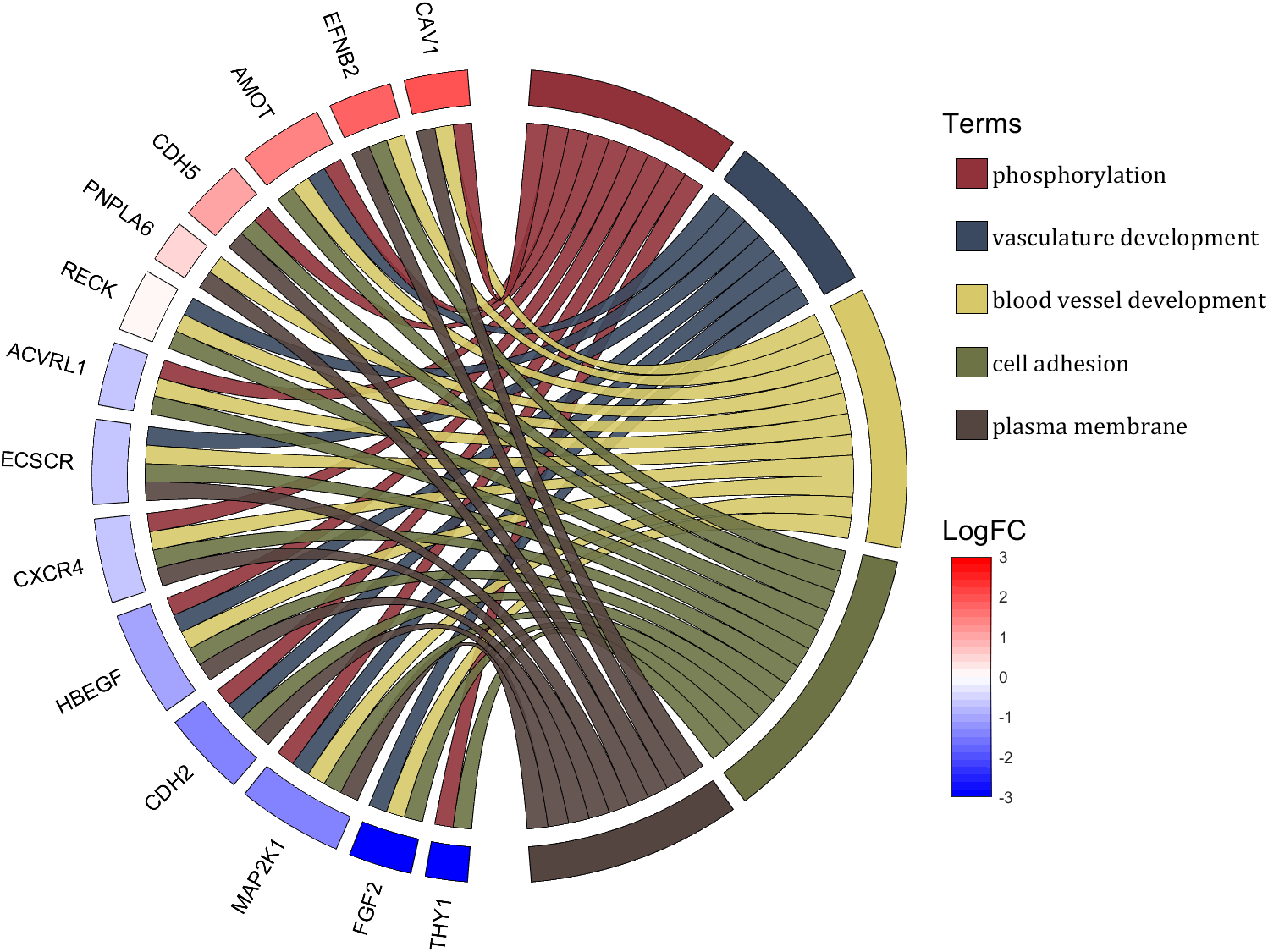
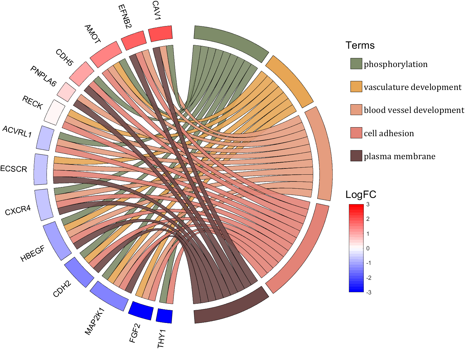
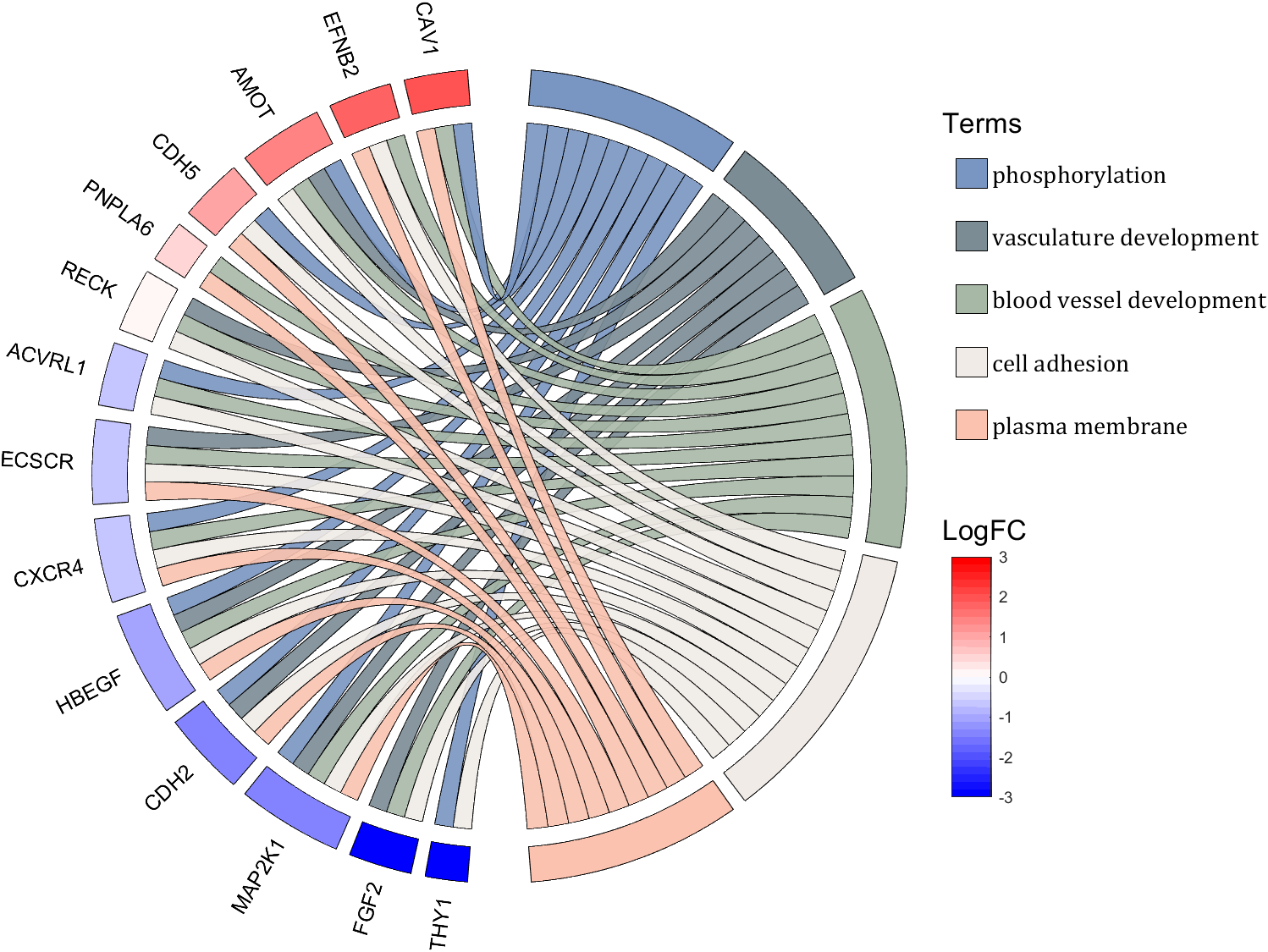
demo 10
rng(2)
dataMat = rand([14,5]) > .3;
colName = {'phosphorylation', 'vasculature development', 'blood vessel development', ...
'cell adhesion', 'plasma membrane'};
rowName = {'THY1', 'FGF2', 'MAP2K1', 'CDH2', 'HBEGF', 'CXCR4', 'ECSCR',...
'ACVRL1', 'RECK', 'PNPLA6', 'CDH5', 'AMOT', 'EFNB2', 'CAV1'};
figure('Units','normalized', 'Position',[.02,.05,.9,.85])
CC = chordChart(dataMat, 'colName',colName, 'rowName',rowName, 'Sep',1/80, 'LRadius',1.2);
CC = CC.draw();
CListT1 = [0.5686 0.1961 0.2275
0.2275 0.2863 0.3765
0.8431 0.7882 0.4118
0.4275 0.4510 0.2706
0.3333 0.2706 0.2510];
CListT2 = [0.4941 0.5490 0.4118
0.9059 0.6510 0.3333
0.8980 0.6157 0.4980
0.8902 0.5137 0.4667
0.4275 0.2824 0.2784];
CListT3 = [0.4745 0.5843 0.7569
0.4824 0.5490 0.5843
0.6549 0.7216 0.6510
0.9412 0.9216 0.9059
0.9804 0.7608 0.6863];
CListT = CListT3;
for i = 1:size(dataMat, 2)
CC.setSquareT_N(i, 'FaceColor',CListT(i,:), 'EdgeColor',[0,0,0])
end
for i = 1:size(dataMat, 1)
for j = 1:size(dataMat, 2)
CC.setChordMN(i,j, 'FaceColor',CListT(j,:), 'FaceAlpha',.9, 'EdgeColor',[0,0,0])
end
end
logFC = sort(rand(1,14))*6 - 3;
for i = 1:size(dataMat, 1)
CC.setSquareF_N(i, 'CData',logFC(i), 'FaceColor','flat', 'EdgeColor',[0,0,0])
end
CMap = [ 0 0 1.0000; 0.0645 0.0645 1.0000; 0.1290 0.1290 1.0000; 0.1935 0.1935 1.0000
0.2581 0.2581 1.0000; 0.3226 0.3226 1.0000; 0.3871 0.3871 1.0000; 0.4516 0.4516 1.0000
0.5161 0.5161 1.0000; 0.5806 0.5806 1.0000; 0.6452 0.6452 1.0000; 0.7097 0.7097 1.0000
0.7742 0.7742 1.0000; 0.8387 0.8387 1.0000; 0.9032 0.9032 1.0000; 0.9677 0.9677 1.0000
1.0000 0.9677 0.9677; 1.0000 0.9032 0.9032; 1.0000 0.8387 0.8387; 1.0000 0.7742 0.7742
1.0000 0.7097 0.7097; 1.0000 0.6452 0.6452; 1.0000 0.5806 0.5806; 1.0000 0.5161 0.5161
1.0000 0.4516 0.4516; 1.0000 0.3871 0.3871; 1.0000 0.3226 0.3226; 1.0000 0.2581 0.2581
1.0000 0.1935 0.1935; 1.0000 0.1290 0.1290; 1.0000 0.0645 0.0645; 1.0000 0 0];
colormap(CMap);
try clim([-3,3]),catch,end
try caxis([-3,3]),catch,end
CBHdl = colorbar();
CBHdl.Position = [0.74,0.25,0.02,0.2];
patchHdl = findobj(gca, 'Type','patch');
for i = 1:length(patchHdl)
tX = patchHdl(i).XData;
tY = patchHdl(i).YData;
patchHdl(i).XData = tY;
patchHdl(i).YData = - tX;
end
txtHdl = findobj(gca, 'Type','text');
for i = 1:length(txtHdl)
txtHdl(i).Position([1,2]) = [1,-1].*txtHdl(i).Position([2,1]);
if txtHdl(i).Position(1) < 0
txtHdl(i).HorizontalAlignment = 'right';
else
txtHdl(i).HorizontalAlignment = 'left';
end
end
lineHdl = findobj(gca, 'Type','line');
for i = 1:length(lineHdl)
tX = lineHdl(i).XData;
tY = lineHdl(i).YData;
lineHdl(i).XData = tY;
lineHdl(i).YData = - tX;
end
txtHdl = findobj(gca, 'Type','text');
for i = 1:length(txtHdl)
if txtHdl(i).Position(1) > 0
txtHdl(i).Visible = 'off';
end
end
text(1.25,-.15, 'LogFC', 'FontSize',16)
text(1.25,1, 'Terms', 'FontSize',16)
patchHdl = [];
for i = 1:size(dataMat, 2)
patchHdl(i) = fill([10,11,12],[10,13,13], CListT(i,:), 'EdgeColor',[0,0,0]);
end
lgdHdl = legend(patchHdl, colName, 'Location','best', 'FontSize',14, 'FontName','Cambria', 'Box','off');
lgdHdl.Position = [.735,.53,.167,.27];
lgdHdl.ItemTokenSize = [18,8];
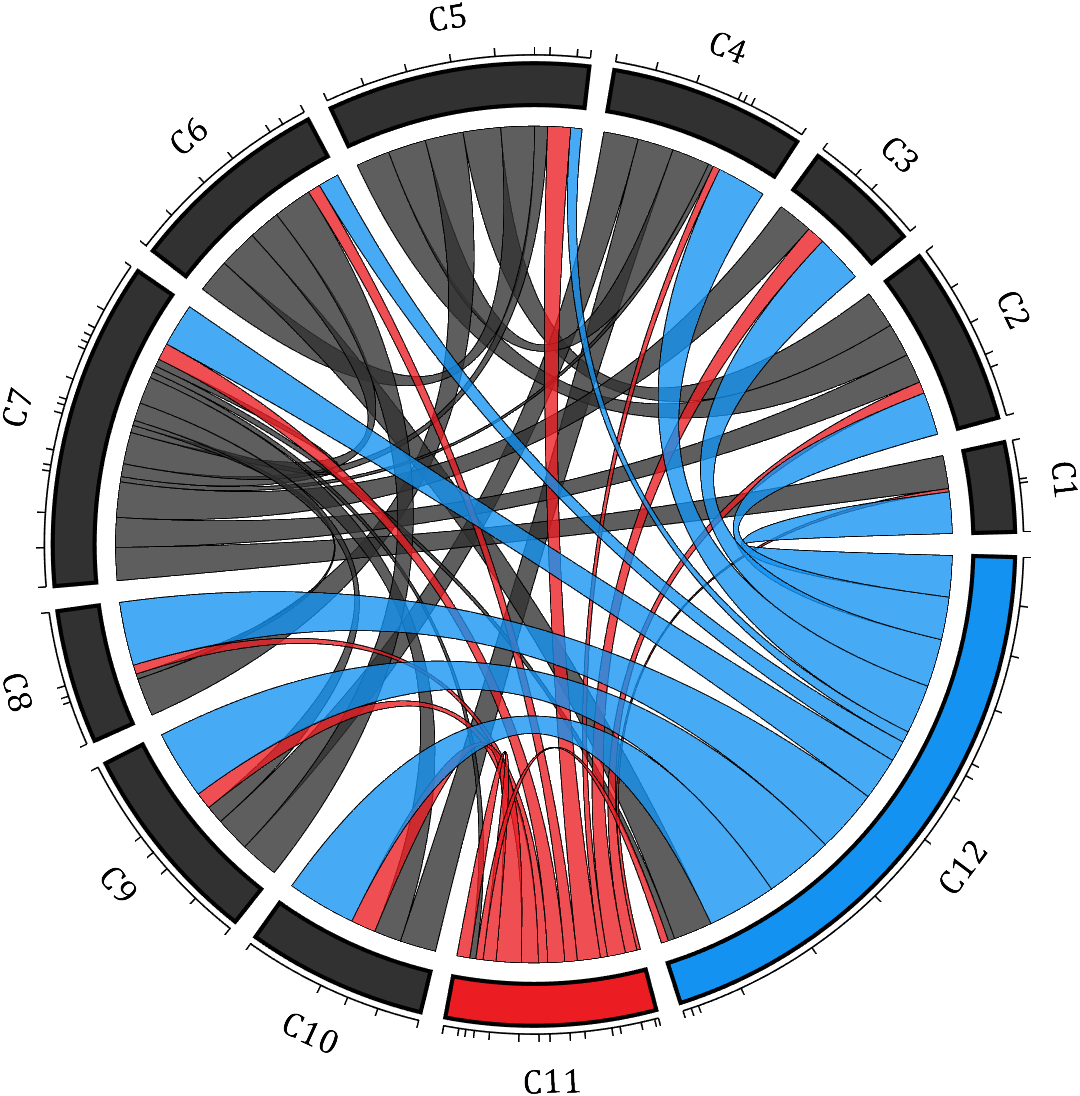
demo 11
rng(2)
dataMat = rand([12,12]);
dataMat(dataMat < .85) = 0;
dataMat(7,:) = 1.*(rand(1,12)+.1);
dataMat(11,:) = .6.*(rand(1,12)+.1);
dataMat(12,:) = [2.*(rand(1,10)+.1), 0, 0];
CList = [repmat([49,49,49],[10,1]); 235,28,34; 19,146,241]./255;
figure('Units','normalized', 'Position',[.02,.05,.6,.85])
BCC = biChordChart(dataMat, 'Arrow','off', 'CData',CList);
BCC = BCC.draw();
BCC.tickState('on')
BCC.setFont('FontName','Cambria', 'FontSize',17)
for i = 1:size(dataMat, 1)
for j = 1:size(dataMat, 2)
if dataMat(i,j) > 0
BCC.setChordMN(i,j, 'FaceAlpha',.78, 'EdgeColor',[0,0,0])
end
end
end
for i = 1:size(dataMat, 1)
BCC.setSquareN(i, 'EdgeColor',[0,0,0], 'LineWidth',2)
end
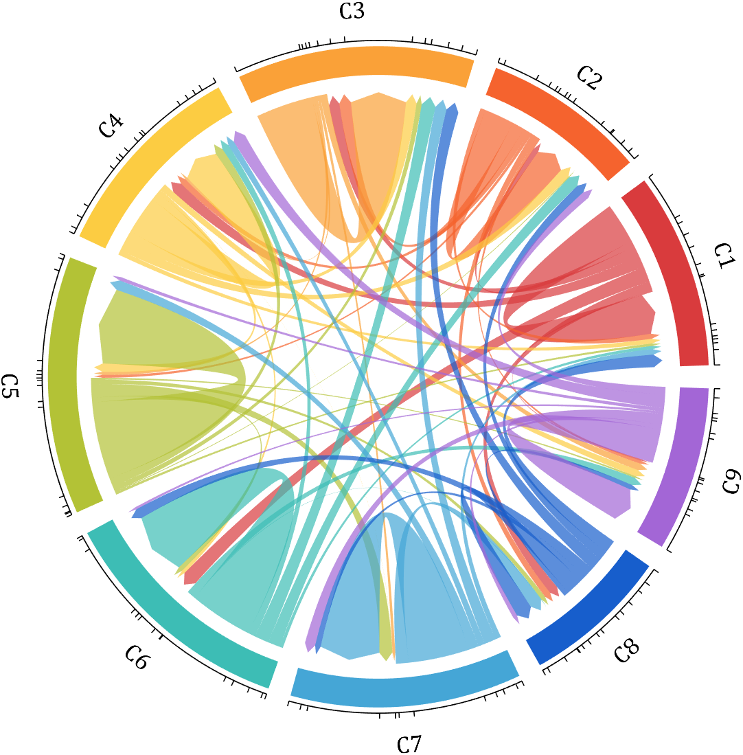
demo 12
dataMat = rand([9,9]);
dataMat(dataMat > .7) = 0;
dataMat(eye(9) == 1) = (rand([1,9])+.2).*3;
CList = [0.85,0.23,0.24
0.96,0.39,0.18
0.98,0.63,0.22
0.99,0.80,0.26
0.70,0.76,0.21
0.24,0.74,0.71
0.27,0.65,0.84
0.09,0.37,0.80
0.64,0.40,0.84];
figure('Units','normalized', 'Position',[.02,.05,.6,.85])
BCC = biChordChart(dataMat, 'Arrow','on', 'CData',CList);
BCC = BCC.draw();
BCC.tickState('on')
BCC.setFont('FontName','Cambria', 'FontSize',17)
for i = 1:size(dataMat, 1)
for j = 1:size(dataMat, 2)
if dataMat(i,j) > 0
BCC.setChordMN(i,j, 'FaceAlpha',.7)
end
end
end
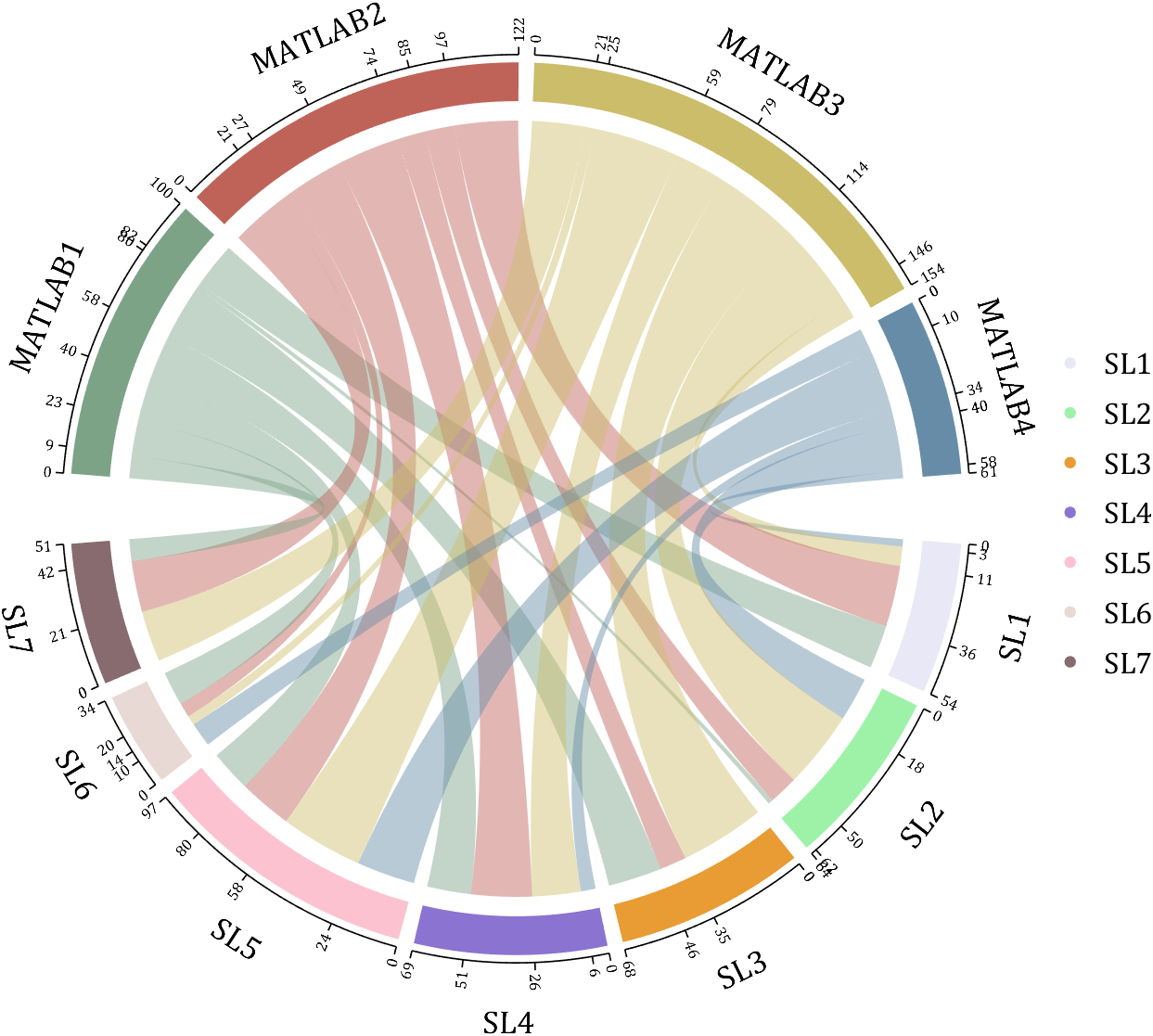
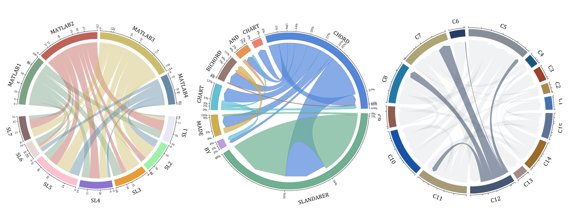
demo 13
rng(2)
dataMat = randi([1,40], [7,4]);
dataMat(rand([7,4]) < .1) = 0;
colName = compose('MATLAB%d', 1:4);
rowName = compose('SL%d', 1:7);
figure('Units','normalized', 'Position',[.02,.05,.7,.85])
CC = chordChart(dataMat, 'rowName',rowName, 'colName',colName, 'Sep',1/80, 'LRadius',1.32);
CC = CC.draw();
CListT = [0.49,0.64,0.53
0.75,0.39,0.35
0.80,0.74,0.42
0.40,0.55,0.66];
for i = 1:size(dataMat, 2)
CC.setSquareT_N(i, 'FaceColor',CListT(i,:))
end
CListF = [0.91,0.91,0.97
0.62,0.95,0.66
0.91,0.61,0.20
0.54,0.45,0.82
0.99,0.76,0.81
0.91,0.85,0.83
0.53,0.42,0.43];
for i = 1:size(dataMat, 1)
CC.setSquareF_N(i, 'FaceColor',CListF(i,:))
end
for i = 1:size(dataMat, 1)
for j = 1:size(dataMat, 2)
CC.setChordMN(i,j, 'FaceColor',CListT(j,:), 'FaceAlpha',.46)
end
end
CC.tickState('on')
CC.tickLabelState('on')
CC.setFont('FontSize',17, 'FontName','Cambria')
CC.setTickFont('FontSize',8, 'FontName','Cambria')
scatterHdl = scatter(10.*ones(size(dataMat,1)),10.*ones(size(dataMat,1)), ...
55, 'filled');
for i = 1:length(scatterHdl)
scatterHdl(i).CData = CListF(i,:);
end
lgdHdl = legend(scatterHdl, rowName, 'Location','best', 'FontSize',16, 'FontName','Cambria', 'Box','off');
set(lgdHdl, 'Position',[.77,.38,.1658,.27])
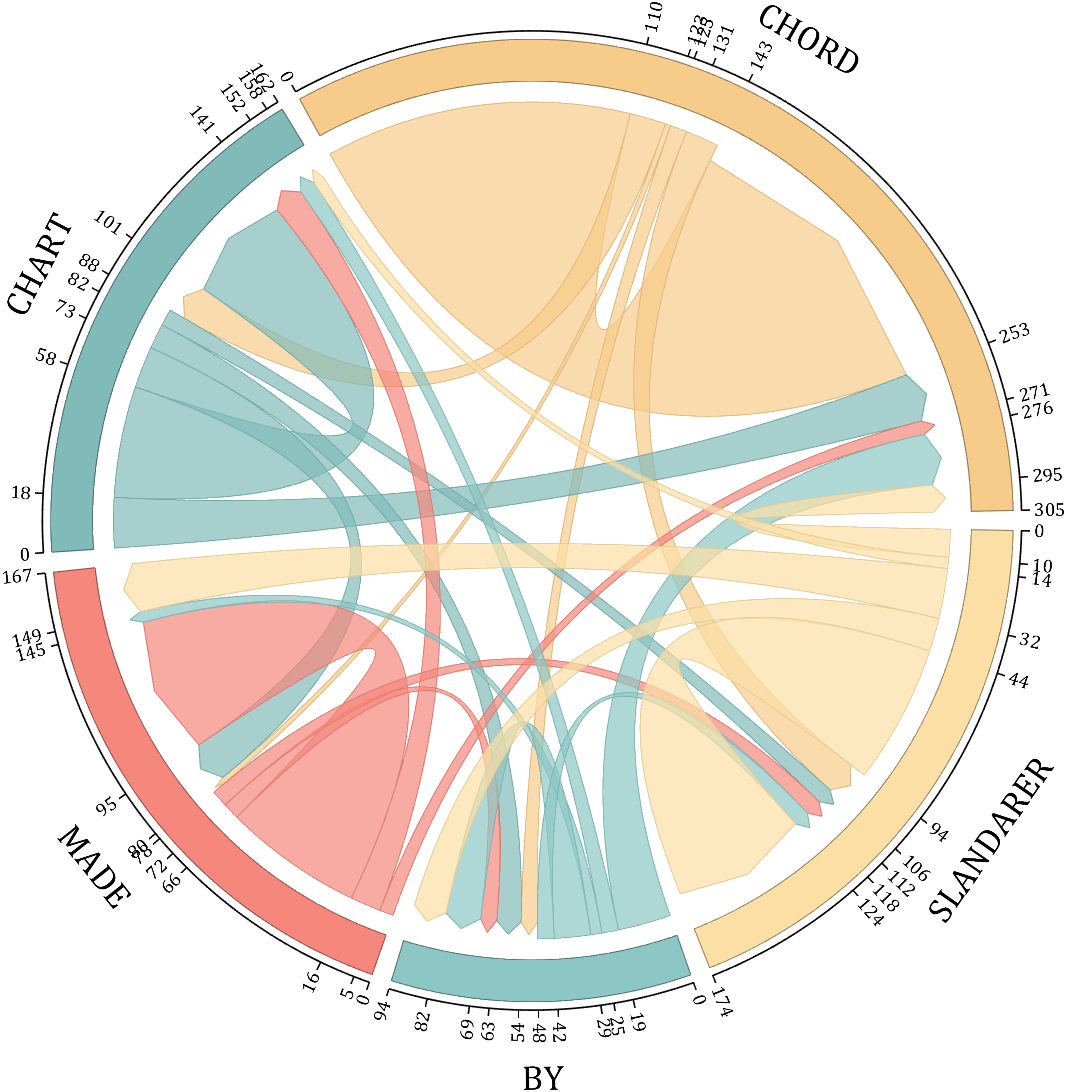
demo 14
rng(6)
dataMat = randi([1,20], [8,8]);
dataMat(dataMat > 5) = 0;
dataMat(1,:) = randi([1,15], [1,8]);
dataMat(1,8) = 40;
dataMat(8,8) = 60;
dataMat = dataMat./sum(sum(dataMat));
CList = [0.33,0.53,0.86
0.94,0.50,0.42
0.92,0.58,0.30
0.59,0.47,0.45
0.37,0.76,0.82
0.82,0.68,0.29
0.75,0.62,0.87
0.43,0.69,0.57];
NameList={'CHORD', 'CHART', 'AND', 'BICHORD',...
'CHART', 'MADE', 'BY', 'SLANDARER'};
figure('Units','normalized', 'Position',[.02,.05,.6,.85])
BCC = biChordChart(dataMat, 'Arrow','on', 'CData',CList, 'Sep',1/12, 'Label',NameList, 'LRadius',1.33);
BCC = BCC.draw();
BCC.tickState('on')
for i = 1:size(dataMat, 1)
for j = 1:size(dataMat, 2)
if dataMat(i,j) > 0
BCC.setChordMN(i,j, 'FaceAlpha',.7, 'EdgeColor',CList(i,:)./1.1)
end
end
end
for i = 1:size(dataMat, 1)
BCC.setSquareN(i, 'EdgeColor',CList(i,:)./1.7)
end
BCC.setFont('FontName','Cambria', 'FontSize',17)
BCC.tickLabelState('on')
BCC.setTickFont('FontName','Cambria', 'FontSize',9)
BCC.setTickLabelFormat(@(x)[num2str(round(x*100)),'%'])
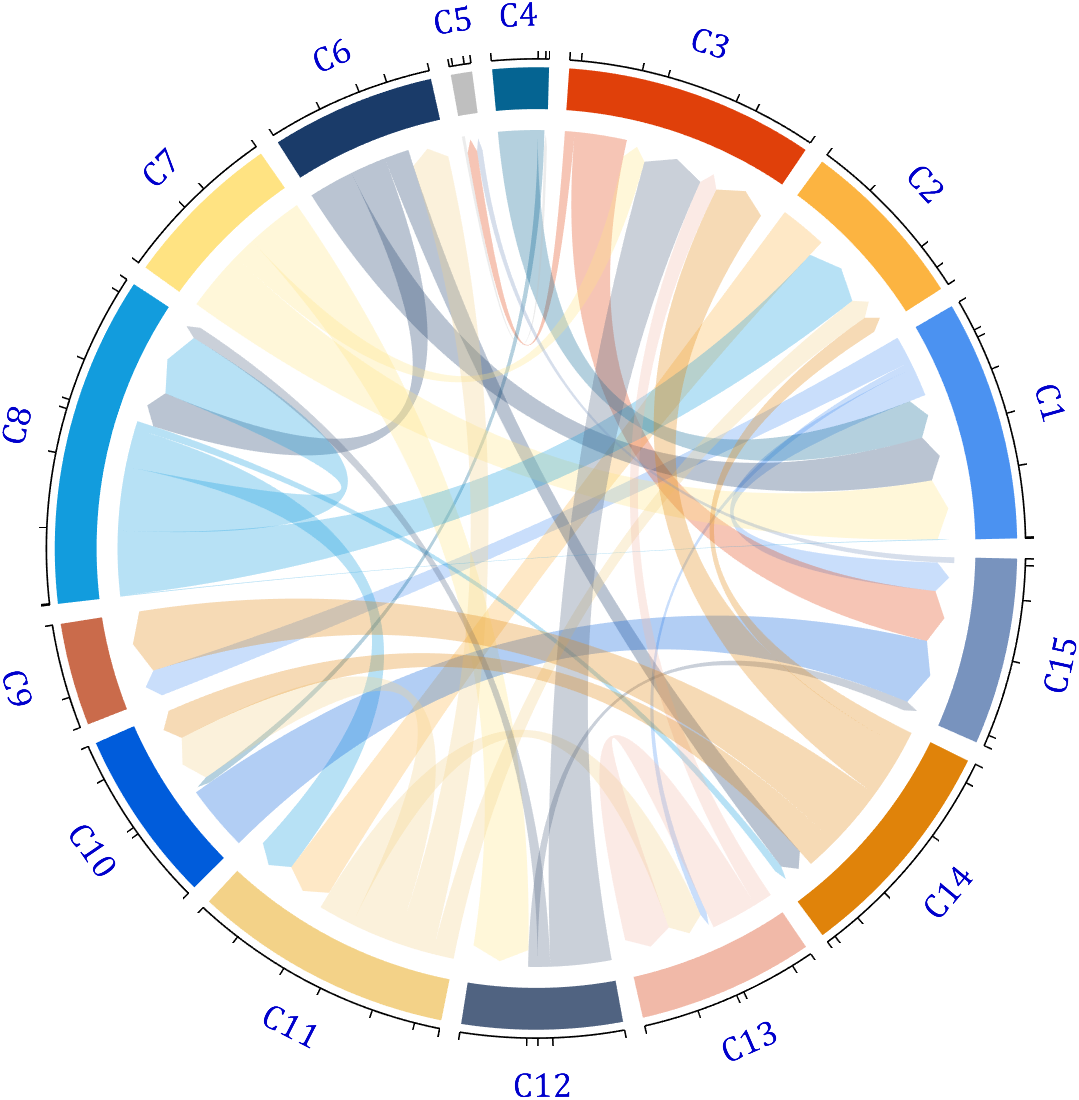
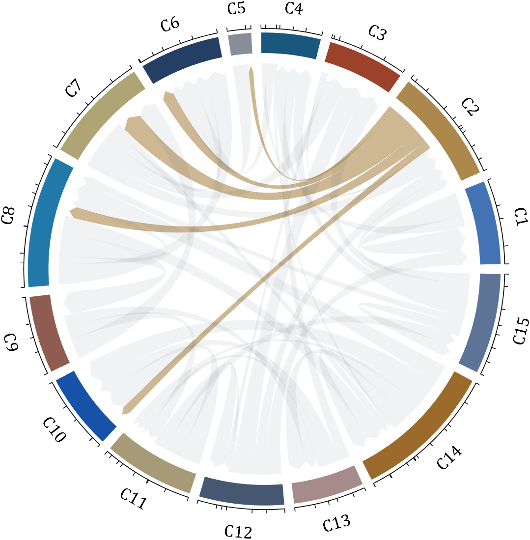
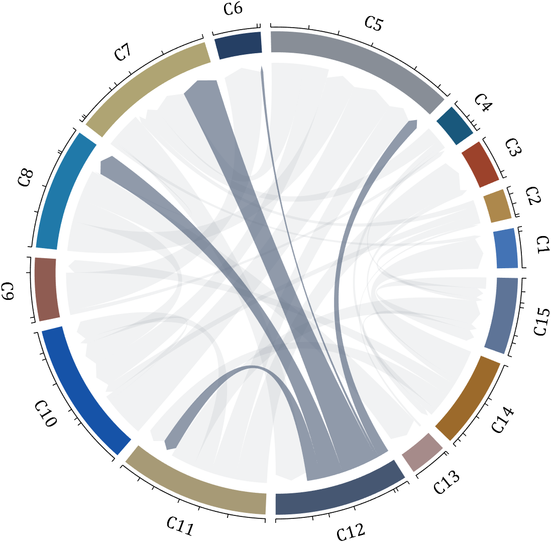
demo 15
CList = [0.81,0.72,0.83
0.69,0.82,0.89
0.17,0.44,0.64
0.70,0.85,0.55
0.03,0.57,0.13
0.97,0.67,0.64
0.84,0.09,0.12
1.00,0.80,0.46
0.98,0.52,0.01
];
figure('Units','normalized', 'Position',[.02,.05,.53,.85], 'Color',[1,1,1])
ax1 = axes('Parent',gcf, 'Position',[0,1/2,1/2,1/2]);
dataMat = rand([9,9]);
dataMat(dataMat > .4) = 0;
BCC = biChordChart(dataMat, 'Arrow','on', 'CData',CList);
BCC = BCC.draw();
BCC.tickState('on')
BCC.setFont('Visible','off')
for i = 1:size(dataMat, 1)
for j = 1:size(dataMat, 2)
if dataMat(i,j) > 0
BCC.setChordMN(i,j, 'FaceAlpha',.6)
end
end
end
text(-1.2,1.2, 'a', 'FontName','Times New Roman', 'FontSize',35)
ax2 = axes('Parent',gcf, 'Position',[1/2,1/2,1/2,1/2]);
dataMat = rand([9,9]);
dataMat(dataMat > .4) = 0;
dataMat = dataMat.*(1:9);
BCC = biChordChart(dataMat, 'Arrow','on', 'CData',CList);
BCC = BCC.draw();
BCC.tickState('on')
BCC.setFont('Visible','off')
for i = 1:size(dataMat, 1)
for j = 1:size(dataMat, 2)
if dataMat(i,j) > 0
BCC.setChordMN(i,j, 'FaceAlpha',.6)
end
end
end
text(-1.2,1.2, 'b', 'FontName','Times New Roman', 'FontSize',35)
ax3 = axes('Parent',gcf, 'Position',[0,0,1/2,1/2]);
dataMat = rand([9,9]);
dataMat(dataMat > .4) = 0;
dataMat = dataMat.*(1:9).';
BCC = biChordChart(dataMat, 'Arrow','on', 'CData',CList);
BCC = BCC.draw();
BCC.tickState('on')
BCC.setFont('Visible','off')
for i = 1:size(dataMat, 1)
for j = 1:size(dataMat, 2)
if dataMat(i,j) > 0
BCC.setChordMN(i,j, 'FaceAlpha',.6)
end
end
end
text(-1.2,1.2, 'c', 'FontName','Times New Roman', 'FontSize',35)
ax4 = axes('Parent',gcf, 'Position',[1/2,0,1/2,1/2]);
ax4.XColor = 'none'; ax4.YColor = 'none';
ax4.XLim = [-1,1]; ax4.YLim = [-1,1];
hold on
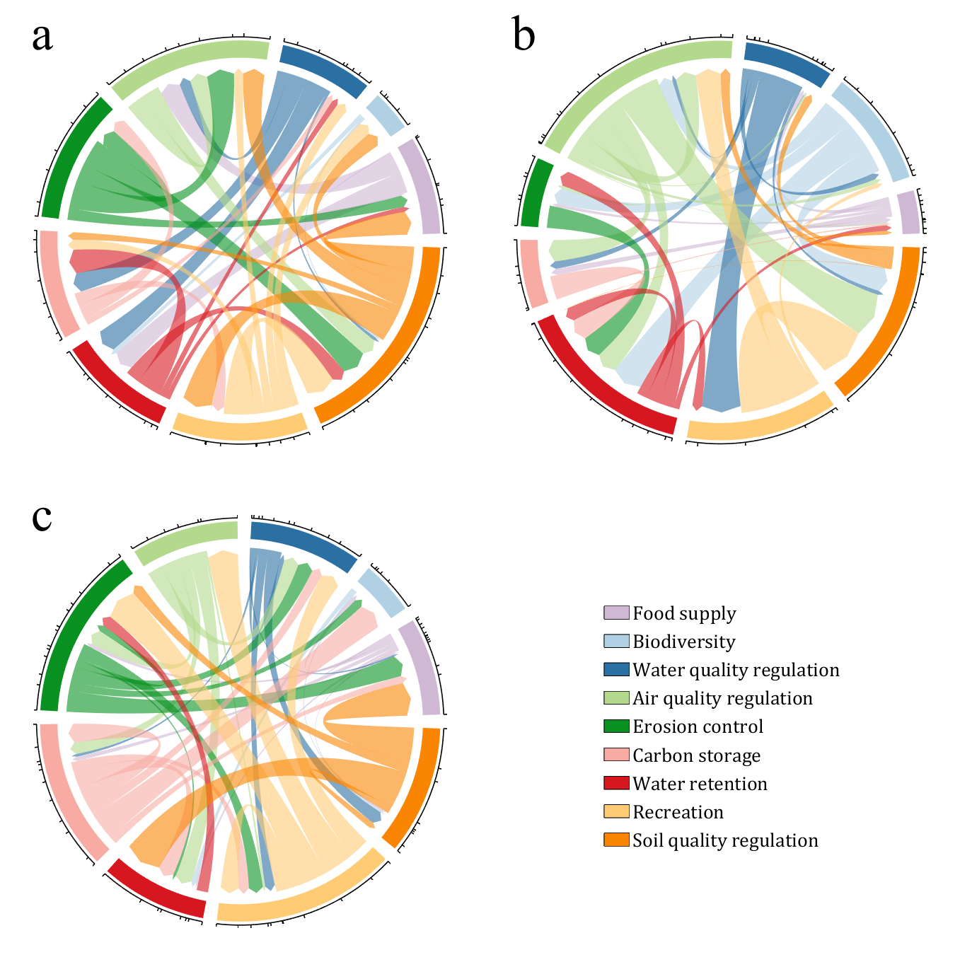
NameList = {'Food supply', 'Biodiversity', 'Water quality regulation', ...
'Air quality regulation', 'Erosion control', 'Carbon storage', ...
'Water retention', 'Recreation', 'Soil quality regulation'};
patchHdl = [];
for i = 1:size(dataMat, 2)
patchHdl(i) = fill([10,11,12],[10,13,13], CList(i,:), 'EdgeColor',[0,0,0]);
end
lgdHdl = legend(patchHdl, NameList, 'Location','best', 'FontSize',14, 'FontName','Cambria', 'Box','off');
lgdHdl.Position = [.625,.11,.255,.27];
lgdHdl.ItemTokenSize = [18,8];
demo 16
dataMat = rand([15,15]);
dataMat(dataMat > .2) = 0;
CList = [ 75,146,241; 252,180, 65; 224, 64, 10; 5,100,146; 191,191,191;
26, 59,105; 255,227,130; 18,156,221; 202,107, 75; 0, 92,219;
243,210,136; 80, 99,129; 241,185,168; 224,131, 10; 120,147,190]./255;
CListC = [54,69,92]./255;
CList = CList.*.6 + CListC.*.4;
figure('Units','normalized', 'Position',[.02,.05,.6,.85])
BCC = biChordChart(dataMat, 'Arrow','on', 'CData',CList);
BCC = BCC.draw();
BCC.tickState('on')
BCC.setFont('FontName','Cambria', 'FontSize',17, 'Color',[0,0,0])
for i = 1:size(dataMat, 1)
for j = 1:size(dataMat, 2)
if dataMat(i,j) > 0
BCC.setChordMN(i,j, 'FaceColor',CListC ,'FaceAlpha',.07)
end
end
end
[~, N] = max(sum(dataMat > 0, 2));
for j = 1:size(dataMat, 2)
BCC.setChordMN(N,j, 'FaceColor',CList(N,:) ,'FaceAlpha',.6)
end
You need to download following tools:


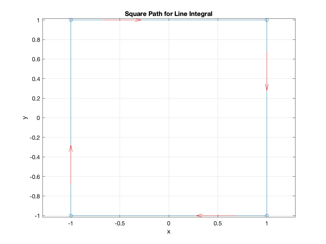
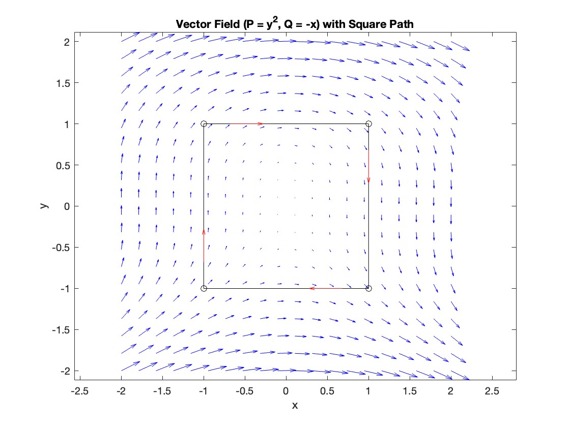
 , where C is the boundary of the square