搜索
I came across this fun video from @Christoper Lum, and I have to admit—his MathWorks swag collection is pretty impressive! He’s got pieces I even don’t have.
So now I’m curious… what MathWorks swag do you have hiding in your office or closet?
- Which one is your favorite?
- Which ones do you want to add to your collection?
Show off your swag and share it with the community! 🚀
The functionality would allow report generation straight from live scripts that could be shared without exposing the code. This could be useful for cases where the recipient of the report only cares about the results and not the code details, or when the methodology is part of a company know how, e.g. Engineering services companies.
In order for it to be practical for use it would also require that variable values could be inserted into the text blocks, e.g. #var_name# would insert the value of the variable "var_name" and possibly selecting which code blocks to be hidden.
Since R2024b, a Levenberg–Marquardt solver (TrainingOptionsLM) was introduced. The built‑in function trainnet now accepts training options via the trainingOptions function (https://www.mathworks.com/help/deeplearning/ref/trainingoptions.html#bu59f0q-2) and supports the LM algorithm. I have been curious how to use it in deep learning, and the official documentation has not provided a concrete usage example so far. Below I give a simple example to illustrate how to use this LM algorithm to optimize a small number of learnable parameters.
For example, consider the nonlinear function:
y_hat = @(a,t) a(1)*(t/100) + a(2)*(t/100).^2 + a(3)*(t/100).^3 + a(4)*(t/100).^4;
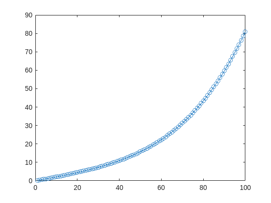
It represents a curve. Given 100 matching points (t → y_hat), we want to use least squares to estimate the four parameters a1–a4.
t = (1:100)';
y_hat = @(a,t)a(1)*(t/100) + a(2)*(t/100).^2 + a(3)*(t/100).^3 + a(4)*(t/100).^4;
x_true = [ 20 ; 10 ; 1 ; 50 ];
y_true = y_hat(x_true,t);
plot(t,y_true,'o-')
- Using the traditional lsqcurvefit-wrapped "Levenberg–Marquardt" algorithm:
x_guess = [ 5 ; 2 ; 0.2 ; -10 ];
options = optimoptions("lsqcurvefit",Algorithm="levenberg-marquardt",MaxFunctionEvaluations=800);
[x,resnorm,residual,exitflag] = lsqcurvefit(y_hat,x_guess,t,y_true,-50*ones(4,1),60*ones(4,1),options);
x,resnorm,exitflag
- Using the deep-learning-wrapped "Levenberg–Marquardt" algorithm:
options = trainingOptions("lm", ...
InitialDampingFactor=0.002, ...
MaxDampingFactor=1e9, ...
DampingIncreaseFactor=12, ...
DampingDecreaseFactor=0.2,...
GradientTolerance=1e-6, ...
StepTolerance=1e-6,...
Plots="training-progress");
numFeatures = 1;
layers = [featureInputLayer(numFeatures,'Name','input')
fitCurveLayer(Name='fitCurve')];
net = dlnetwork(layers);
XData = dlarray(t);
YData = dlarray(y_true);
netTrained = trainnet(XData,YData,net,"mse",options);
netTrained.Layers(2)
classdef fitCurveLayer < nnet.layer.Layer ...
& nnet.layer.Acceleratable
% Example custom SReLU layer.
properties (Learnable)
% Layer learnable parameters
a1
a2
a3
a4
end
methods
function layer = fitCurveLayer(args)
arguments
args.Name = "lm_fit";
end
% Set layer name.
layer.Name = args.Name;
% Set layer description.
layer.Description = "fit curve layer";
end
function layer = initialize(layer,~)
% layer = initialize(layer,layout) initializes the layer
% learnable parameters using the specified input layout.
if isempty(layer.a1)
layer.a1 = rand();
end
if isempty(layer.a2)
layer.a2 = rand();
end
if isempty(layer.a3)
layer.a3 = rand();
end
if isempty(layer.a4)
layer.a4 = rand();
end
end
function Y = predict(layer, X)
% Y = predict(layer, X) forwards the input data X through the
% layer and outputs the result Y.
% Y = layer.a1.*exp(-X./layer.a2) + layer.a3.*X.*exp(-X./layer.a4);
Y = layer.a1*(X/100) + layer.a2*(X/100).^2 + layer.a3*(X/100).^3 + layer.a4*(X/100).^4;
end
end
end
The network is very simple — only the fitCurveLayer defines the learnable parameters a1–a4. I observed that the output values are very close to those from lsqcurvefit.
I saw this YouTube short on my feed: What is MATLab?

I was mostly mesmerized by the minecraft gameplay going on in the background.
Found it funny, thought i'd share.
Trinity
- It's the question that drives us, Neo. It's the question that brought you here. You know the question, just as I did.
Neo
- What is the Matlab?
Morpheus
- Unfortunately, no one can be told what the Matlab is. You have to see it for yourself.
And also later :
Morpheus
- The Matlab is everywhere. It is all around us. Even now, in this very room. You can feel it when you go to work [...]
The Architect
- The first Matlab I designed was quite naturally perfect. It was a work of art. Flawless. Sublime.
[My Matlab quotes version of the movie (Matrix, 1999) ]
Modern engineering requires both robust hardware and powerful simulation tools. MATLAB and Simulink are widely used for data analysis, control design, and embedded system development. At the same time, Kasuo offers a wide range of components—from sensors and connectors to circuit protection devices—that engineers rely on to build real-world systems.
By combining these tools, developers can bridge the gap between simulation and implementation, ensuring their designs are reliable and ready for deployment.
Example Use Case: Sensor Data Acquisition and Processing
- Kasuo Hardware Setup
- Select a Kasuo sensor (e.g., temperature, microphone, or motion sensor).
- Connect it to a DAQ or microcontroller board for data collection.
- Data Acquisition in MATLAB
- Use MATLAB’s Data Acquisition Toolbox to stream sensor data directly.
- Example snippet:
s = daq("ni");
addinput(s,
"Dev1", "ai0", "Voltage");
data = read(s, seconds(
5), "OutputFormat", "Matrix");
plot(data);
- Signal Processing with Simulink
- Build a Simulink model to filter noise, detect anomalies, or design control logic.
- Simulink enables real-time visualization and iterative tuning.
- Validation & Protection Simulation
- Add Kasuo’s circuit protection components (e.g., TVS diodes, surge suppressors) in the physical design.
- Use Simulink to simulate stress conditions, validating system robustness before hardware testing.
Benefits of the Workflow
- Faster prototyping with MATLAB & Simulink.
- Greater reliability by incorporating Kasuo protection devices.
- Seamless transition from model to hardware implementation.
Conclusion
Kasuo’s electronic components provide the hardware foundation for many embedded and signal processing applications. When combined with MATLAB and Simulink, engineers can design, simulate, and validate systems more efficiently—reducing risks and development time.
With AI agents dev coding on other languages has become so easy.
Im waiting for matlab to build something like warp but for matlab.
I know they have the current ai but with all respect it's rubbish compared to vibe coding tools in others sectors.
Matlab leads AI so it really should be leading this space.
Function Syntax Design Conundrum
As a MATLAB enthusiast, I particularly enjoy Steve Eddins' blog and the cool things he explores. MATLAB's new argument blocks are great, but there's one frustrating limitation that Steve outlined beautifully in his blog post "Function Syntax Design Conundrum": cases where an argument should accept both enumerated values AND other data types.
Steve points out this could be done using the input parser, but I prefer having tab completions and I'm not a fan of maintaining function signature JSON files for all my functions.
Personal Context on Enumerations
To be clear: I honestly don't like enumerations in any way, shape, or form. One reason is how awkward they are. I've long suspected they're simply predefined constructor calls with a set argument, and I think that's all but confirmed here. This explains why I've had to fight the enumeration system when trying to take arguments of many types and normalize them to enumerated members, or have numeric values displayed as enumerated members without being recast to the superclass every operation.
The Discovery
While playing around extensively with metadata for another project, I realized (and I'm entirely unsure why it took so long) that the properties of a metaclass object are just, in many cases, the attributes of the classdef. In this realization, I found a solution to Steve's and my problem.
To be clear: I'm not in love with this solution. I would much prefer a better approach for allowing variable sets of membership validation for arguments. But as it stands, we don't have that, so here's an interesting, if incredibly hacky, solution.
If you call struct() on a metaclass object to view its hidden properties, you'll notice that in addition to the public "Enumeration" property, there's a hidden "Enumerable" property. They're both logicals, which implies they're likely functionally distinct. I was curious about that distinction and hoped to find some functionality by intentionally manipulating these values - and I did, solving the exact problem Steve mentions.
The Problem Statement
We have a function with an argument that should allow "dual" input types: enumerated values (Steve's example uses days of the week, mine uses the "all" option available in various dimension-operating functions) AND integers. We want tab completion for the enumerated values while still accepting the numeric inputs.
A Solution for Tab-Completion Supported Arguments
Rather than spoil Steve's blog post, let me use my own example: implementing a none() function. The definition is simple enough tf = ~any(A, dim); but when we wrap this in another function, we lose the tab-completion that any() provides for the dim argument (which gives you "all"). There's no great way to implement this as a function author currently - at least, that's well documented.
So here's my solution:
%% Example Function Implementation
% This is a simple implementation of the DimensionArgument class for implementing dual type inputs that allow enumerated tab-completion.
function tf = none(A, dim)
arguments(Input)
A logical;
dim DimensionArgument = DimensionArgument(A, true);
end
% Simple example (notice the use of uplus to unwrap the hidden property)
tf = ~any(A, +dim);
end
I like this approach because the additional work required to implement it, once the enumeration class is initialized, is minimal. Here are examples of function calls, note that the behavior parallels that of the MATLAB native-style tab-completion:
%% Test Data
% Simple logical array for testing
A = randi([0, 1], [3, 5], "logical");
%% Example function calls
tf = none(A, "all"); % This is the tab-completion it's 1:1 with MATLABs behavior
tf = none(A, [1, 2]); % We can still use valid arguments (validated in the constructor)
tf = none(A); % Showcase of the constructors use as a default argument generator
How It Works
What makes this work is the previously mentioned Enumeration attribute. By setting Enumeration = false while still declaring an enumeration block in the classdef file, we get the suggested members as auto-complete suggestions. As I hinted at, the value of enumerations (if you don't subclass a builtin and define values with the someMember (1) syntax) are simply arguments to constructor calls.
We also get full control over the storage and handling of the class, which means we lose the implicit storage that enumerations normally provide and are responsible for doing so ourselves - but I much prefer this. We can implement internal validation logic to ensure values that aren't in the enumerated set still comply with our constraints, and store the input (whether the enumerated member or alternative type) in an internal property.
As seen in the example class below, this maintains a convenient interface for both the function caller and author the only particuarly verbose portion is the conversion methods... Which if your willing to double down on the uplus unwrapping context can be avoided. What I have personally done is overload the uplus function to return the input (or perform the identity property) this allowss for the uplus to be used universally to unwrap inputs and for those that cant, and dont have a uplus definition, the value itself is just returned:
classdef(Enumeration = false) DimensionArgument % < matlab.mixin.internal.MatrixDisplay
%DimensionArgument Enumeration class to provide auto-complete on functions needing the dimension type seen in all()
% Enumerations are just macros to make constructor calls with a known set of arguments. Declaring the 'all'
% enumeration member means this class can be set as the type for an input and the auto-completion for the given
% argument will show the enumeration members, allowing tab-completion. Declaring the Enumeration attribute of
% the class as false gives us control over the constructor and internal implementation. As such we can use it
% to validate the numeric inputs, in the event the 'all' option was not used, and return an object that will
% then work in place of valid dimension argument options.
%% Enumeration members
% These are the auto-complete options you'd like to make available for the function signature for a given
% argument.
enumeration(Description="Enumerated value for the dimension argument.")
all
end
%% Properties
% The internal property allows the constructor's input to be stored; this ensures that the value is store and
% that the output of the constructor has the class type so that the validation passes.
% (Constructors must return the an object of the class they're a constructor for)
properties(Hidden, Description="Storage of the constructor input for later use.")
Data = [];
end
%% Constructor method
% By the magic of declaring (Enumeration = false) in our class def arguments we get full control over the
% constructor implementation.
%
% The second argument in this specific instance is to enable the argument's default value to be set in the
% arguments block itself as opposed to doing so in the function body... I like this better but if you didn't
% you could just as easily keep the constructor simple.
methods
function obj = DimensionArgument(A, Adim)
%DimensionArgument Initialize the dimension argument.
arguments
% This will be the enumeration member name from auto-completed entries, or the raw user input if not
% used.
A = [];
% A flag that indicates to create the value using different logic, in this case the first non-singleton
% dimension, because this matches the behavior of functions like, all(), sum() prod(), etc.
Adim (1, 1) logical = false;
end
if(Adim)
% Allows default initialization from an input to match the aforemention function's behavior
obj.Data = firstNonscalarDim(A);
else
% As a convenience for this style of implementation we can validate the input to ensure that since we're
% suppose to be an enumeration, the input is valid
DimensionArgument.mustBeValidMember(A);
% Store the input in a hidden property since declaring ~Enumeration means we are responsible for storing
% it.
obj.Data = A;
end
end
end
%% Conversion methods
% Applies conversion to the data property so that implicit casting of functions works. Unfortunately most of
% the MathWorks defined functions use a different system than that employed by the arguments block, which
% defers to the class defined converter methods... Which is why uplus (+obj) has been defined to unwrap the
% data for ease of use.
methods
function obj = uplus(obj)
obj = obj.Data;
end
function str = char(obj)
str = char(obj.Data);
end
function str = cellstr(obj)
str = cellstr(obj.Data);
end
function str = string(obj)
str = string(obj.Data);
end
function A = double(obj)
A = double(obj.Data);
end
function A = int8(obj)
A = int8(obj.Data);
end
function A = int16(obj)
A = int16(obj.Data);
end
function A = int32(obj)
A = int32(obj.Data);
end
function A = int64(obj)
A = int64(obj.Data);
end
end
%% Validation methods
% These utility methods are for input validation
methods(Static, Access = private)
function tf = isValidMember(obj)
%isValidMember Checks that the input is a valid dimension argument.
tf = (istext(obj) && all(obj == "all", "all")) || (isnumeric(obj) && all(isint(obj) & obj > 0, "all"));
end
function mustBeValidMember(obj)
%mustBeValidMember Validates that the input is a valid dimension argument for the dim/dimVec arguments.
if(~DimensionArgument.isValidMember(obj))
exception("JB:DimensionArgument:InvalidInput", "Input must be an integer value or the term 'all'.")
end
end
end
%% Convenient data display passthrough
methods
function disp(obj, name)
arguments
obj DimensionArgument
name string {mustBeScalarOrEmpty} = [];
end
% Dispatch internal data's display implementation
display(obj.Data, char(name));
end
end
end
In the event you'd actually play with theres here are the function definitions for some of the utility functions I used in them, including my exception would be a pain so i wont, these cases wont use it any...
% Far from my definition isint() but is consistent with mustBeInteger() for real numbers but will suffice for the example
function tf = isint(A)
arguments
A {mustBeNumeric(A)};
end
tf = floor(A) == A
end
% Sort of the same but its fine
function dim = firstNonscalarDim(A)
arguments
A
end
dim = [find(size(A) > 1, 1), 0];
dim(1) = dim(1);
end
Hello MATLAB Central, this is my first article.
My name is Yann. And I love MATLAB.
I also love HTTP (i know, weird fetish)
So i started a conversation with ChatGPT about it:
gitclone('https://github.com/yanndebray/HTTP-with-MATLAB');
cd('HTTP-with-MATLAB')
http_with_MATLAB
I'm not sure that this platform is intended to clone repos from github, but i figured I'd paste this shortcut in case you want to try out my live script http_with_MATLAB.m
A lot of what i program lately relies on external web services (either for fetching data, or calling LLMs).
So I wrote a small tutorial of the 7 or so things I feel like I need to remember when making HTTP requests in MATLAB.
Let me know what you think

I designed and stitched this last week! It uses a total of 20 DMC thread colors, and I frequently stitched with two colors at once to create the gradient.
When you compare MATLAB Plot Gallery with matplotlib gallery, you can see that matplotlib gallery contains a lot of nice graphs which are easy to create in MATLAB but not listed in MATLAB Plot Gallery.
For example, "Data Distribution Plots" section in the MATLAB Plot Gallery includes example for pie function instead of examples for piechart and donutchart functions, etc.
Did you know that function double with string vector input significantly outperforms str2double with the same input:
x = rand(1,50000);
t = string(x);
tic; str2double(t); toc
tic; I1 = str2double(t); toc
tic; I2 = double(t); toc
isequal(I1,I2)
Recently I needed to parse numbers from text. I automatically tried to use str2double. However, profiling revealed that str2double was the main bottleneck in my code. Than I realized that there is a new note (since R2024a) in the documentation of str2double:
"Calling string and then double is recommended over str2double because it provides greater flexibility and allows vectorization. For additional information, see Alternative Functionality."
mlapp being a binary is a pain point for source control. It means that you either have to:
- have hooks in your source control system to zip/unzip a mlapp. However, The Mathworks have informed users not to rely on this as the mlapp format may change.
- do all your source control in MATLAB. This is non standard behaviour. Source code and source control should be independent of each other. Web front-ends to source control systems, 3rd party source control apps, CI/CD systems and much more are extremely limited in what they can do with mlapps.
I wish an mlapp could just be a directory full of the required text/other files.
Requested to post this here from reddit.
There is no call to rescan audio devices in audioPlayerRecorder, even though PortAudio has such a call. I have a measurement environment that takes a long time to initialise. If I forget to plug in my audio device, I have to do it all over again...
Share your ideas, suggestions, and wishlists for improving MathWorks products. What would make the software absolutely perfect for you? Discuss your idea(s) with other community users.
Guidelines & Tips
We encourage all ideas, big or small! To help everyone understand and discuss your suggestion, please include as much detail as possible in your post:
- Product or Feature: Clearly state which product (e.g., MATLAB, Simulink, a toolbox, etc.) or specific feature your idea relates to.
- The Problem or Opportunity: Briefly describe what challenge you’re facing or what opportunity you see for improvement.
- Your Idea: Explain your suggestion in detail. What would you like to see added, changed, or improved? How would it help you and other users?
- Examples or Use Cases (optional): If possible, include an example, scenario, or workflow to illustrate your idea.
- Related Posts (optional): If you’ve seen similar ideas or discussions, feel free to link to them for context.
Ready to share your idea?
Click here and then "Start a Discussion”, and let the community know how MATLAB could be even better for you!
Thank you for your contributions and for helping make MATLAB Central a vibrant place for sharing and improving ideas.
Resharing a fun short video explaining what MATLAB is. :)
t = turtle(); % Start a turtle
t.forward(100); % Move forward by 100
t.backward(100); % Move backward by 100
t.left(90); % Turn left by 90 degrees
t.right(90); % Tur right by 90 degrees
t.goto(100, 100); % Move to (100, 100)
t.turnto(90); % Turn to 90 degrees, i.e. north
t.speed(1000); % Set turtle speed as 1000 (default: 500)
t.pen_up(); % Pen up. Turtle leaves no trace.
t.pen_down(); % Pen down. Turtle leaves a trace again.
t.color('b'); % Change line color to 'b'
t.begin_fill(FaceColor, EdgeColor, FaceAlpha); % Start filling
t.end_fill(); % End filling
t.change_icon('person.png'); % Change the icon to 'person.png'
t.clear(); % Clear the Axes
classdef turtle < handle
properties (GetAccess = public, SetAccess = private)
x = 0
y = 0
q = 0
end
properties (SetAccess = public)
speed (1, 1) double = 500
end
properties (GetAccess = private)
speed_reg = 100
n_steps = 20
ax
l
ht
im
is_pen_up = false
is_filling = false
fill_color
fill_alpha
end
methods
function obj = turtle()
figure(Name='MATurtle', NumberTitle='off')
obj.ax = axes(box="on");
hold on,
obj.ht = hgtransform();
icon = flipud(imread('turtle.png'));
obj.im = imagesc(obj.ht, icon, ...
XData=[-30, 30], YData=[-30, 30], ...
AlphaData=(255 - double(rgb2gray(icon)))/255);
obj.l = plot(obj.x, obj.y, 'k');
obj.ax.XLim = [-500, 500];
obj.ax.YLim = [-500, 500];
obj.ax.DataAspectRatio = [1, 1, 1];
obj.ax.Toolbar.Visible = 'off';
disableDefaultInteractivity(obj.ax);
end
function home(obj)
obj.x = 0;
obj.y = 0;
obj.ht.Matrix = eye(4);
end
function forward(obj, dist)
obj.step(dist);
end
function backward(obj, dist)
obj.step(-dist)
end
function step(obj, delta)
if numel(delta) == 1
delta = delta*[cosd(obj.q), sind(obj.q)];
end
if obj.is_filling
obj.fill(delta);
else
obj.move(delta);
end
end
function goto(obj, x, y)
dx = x - obj.x;
dy = y - obj.y;
obj.turnto(rad2deg(atan2(dy, dx)));
obj.step([dx, dy]);
end
function left(obj, q)
obj.turn(q);
end
function right(obj, q)
obj.turn(-q);
end
function turnto(obj, q)
obj.turn(obj.wrap_angle(q - obj.q, -180));
end
function pen_up(obj)
if obj.is_filling
warning('not available while filling')
return
end
obj.is_pen_up = true;
end
function pen_down(obj, go)
if obj.is_pen_up
if nargin == 1
obj.l(end+1) = plot(obj.x, obj.y, Color=obj.l(end).Color);
else
obj.l(end+1) = go;
end
uistack(obj.ht, 'top')
end
obj.is_pen_up = false;
end
function color(obj, line_color)
if obj.is_filling
warning('not available while filling')
return
end
obj.pen_up();
obj.pen_down(plot(obj.x, obj.y, Color=line_color));
end
function begin_fill(obj, FaceColor, EdgeColor, FaceAlpha)
arguments
obj
FaceColor = [.6, .9, .6];
EdgeColor = [0 0.4470 0.7410];
FaceAlpha = 1;
end
if obj.is_filling
warning('already filling')
return
end
obj.fill_color = FaceColor;
obj.fill_alpha = FaceAlpha;
obj.pen_up();
obj.pen_down(patch(obj.x, obj.y, [1, 1, 1], ...
EdgeColor=EdgeColor, FaceAlpha=0));
obj.is_filling = true;
end
function end_fill(obj)
if ~obj.is_filling
warning('not filling now')
return
end
obj.l(end).FaceColor = obj.fill_color;
obj.l(end).FaceAlpha = obj.fill_alpha;
obj.is_filling = false;
end
function change_icon(obj, filename)
icon = flipud(imread(filename));
obj.im.CData = icon;
obj.im.AlphaData = (255 - double(rgb2gray(icon)))/255;
end
function clear(obj)
obj.x = 0;
obj.y = 0;
delete(obj.ax.Children(2:end));
obj.l = plot(0, 0, 'k');
obj.ht.Matrix = eye(4);
end
end
methods (Access = private)
function animated_step(obj, delta, q, initFcn, updateFcn)
arguments
obj
delta
q
initFcn = @() []
updateFcn = @(~, ~) []
end
dx = delta(1)/obj.n_steps;
dy = delta(2)/obj.n_steps;
dq = q/obj.n_steps;
pause_duration = norm(delta)/obj.speed/obj.speed_reg;
initFcn();
for i = 1:obj.n_steps
updateFcn(dx, dy);
obj.ht.Matrix = makehgtform(...
translate=[obj.x + dx*i, obj.y + dy*i, 0], ...
zrotate=deg2rad(obj.q + dq*i));
pause(pause_duration)
drawnow limitrate
end
obj.x = obj.x + delta(1);
obj.y = obj.y + delta(2);
end
function obj = turn(obj, q)
obj.animated_step([0, 0], q);
obj.q = obj.wrap_angle(obj.q + q, 0);
end
function move(obj, delta)
initFcn = @() [];
updateFcn = @(dx, dy) [];
if ~obj.is_pen_up
initFcn = @() initializeLine();
updateFcn = @(dx, dy) obj.update_end_point(obj.l(end), dx, dy);
end
function initializeLine()
obj.l(end).XData(end+1) = obj.l(end).XData(end);
obj.l(end).YData(end+1) = obj.l(end).YData(end);
end
obj.animated_step(delta, 0, initFcn, updateFcn);
end
function obj = fill(obj, delta)
initFcn = @() initializePatch();
updateFcn = @(dx, dy) obj.update_end_point(obj.l(end), dx, dy);
function initializePatch()
obj.l(end).Vertices(end+1, :) = obj.l(end).Vertices(end, :);
obj.l(end).Faces = 1:size(obj.l(end).Vertices, 1);
end
obj.animated_step(delta, 0, initFcn, updateFcn);
end
end
methods (Static, Access = private)
function update_end_point(l, dx, dy)
l.XData(end) = l.XData(end) + dx;
l.YData(end) = l.YData(end) + dy;
end
function q = wrap_angle(q, min_angle)
q = mod(q - min_angle, 360) + min_angle;
end
end
end
Nice to have - function output argument provide code assist when said function is called
This is a feature which doesn't apear to currently exist, but I think alot of matlab users would like, particularly ones who write alot of custom classes.
Imagine i have a custom class with some properties:
classdef CustomClass < handle
properties
name (1,1) string = "default name"
varOne (1,1) double = 0
end
methods
function obj = CustomClass(name,varOne)
obj.name = name;
obj.VarOne = varOne;
end
end
end
Then imagine I have a function which returns one of these custom class objects:
function [obj] = Calculation(Var1,Var2,name)
arguments (Input)
Var1 (1,1) double
Var2 (1,1) double
end
arguments (Output)
obj (1,1) CustomClass
end
results = Var1 + Var2;
obj = CustomClass(name,result);
end
With this class and this function which returns one of these class objects, I would like the fact that I provided "(1,1) CustomClass" in the output arguemnts block of function "Calculation(Var1,Var2,name)" to trigger code assist automaticaly show me, when writing code that the retuned value from this funciton has properties "name" and "varOne" in the object.
For istance, if I write the following code with this function and the class in the Matlab search path
testObj = Calculation(1,1,"test");
testObj.varOne = 10; %the property "varOne" doesn't apear in code assist when writing this line of code
I would like that the fact function "Calcuation(Var1,Var2,name) has the output arguments block enforcing that this function must return an object of "CustomClass" to make code assist recognise that "testObj" is a "CustomClass" object, just as if testObj was an input argument to another function which had an input argument requiring that "testObj" was a "CustomClass" object.
Maybe this is a feature that may be added to matlab in future releases? (please and thank you LOL)