主要内容
搜索
There will be a warning when we try to solve equations with piecewise:
syms x y
a = x+y;
b = 1.*(x > 0) + 2.*(x <= 0);
eqns = [a + b*x == 1, a - b == 2];
S = solve(eqns, [x y]);
% 错误使用 mupadengine/feval_internal
% System contains an equation of an unknown type.
%
% 出错 sym/solve (第 293 行)
% sol = eng.feval_internal('solve', eqns, vars, solveOptions);
%
% 出错 demo3 (第 5 行)
% S=solve(eqns,[x y]);
But I found that the solve function can include functions such as heaviside to indicate positive and negative:
syms x y
a = x+y;
b = floor(heaviside(x)) - 2*abs(2*heaviside(x) - 1) + 2*floor(-heaviside(x)) + 4;
eqns = [a + b*x == 1, a - b == 2];
S = solve(eqns, [x y])
% S =
% 包含以下字段的 struct:
%
% x: -3/2
% y: 11/2
The piecewise function is divided into two sections, which is so complex, so this work must be encapsulated as a function to complete:
function pwFunc=piecewiseSym(x,waypoint,func,pfunc)
% @author : slandarer
gSign=[1,heaviside(x-waypoint)*2-1];
lSign=[heaviside(waypoint-x)*2-1,1];
inSign=floor((gSign+lSign)/2);
onSign=1-abs(gSign(2:end));
inFunc=inSign.*func;
onFunc=onSign.*pfunc;
pwFunc=simplify(sum(inFunc)+sum(onFunc));
end
Function Introduction
- x : Argument
- waypoint : Segmentation point of piecewise function
- func : Functions on each segment
- pfunc : The value at the segmentation point
example
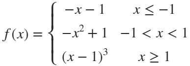
syms x
% x waypoint func pfunc
f=piecewiseSym(x,[-1,1],[-x-1,-x^2+1,(x-1)^3],[-x-1,(x-1)^3]);
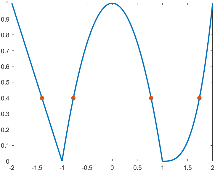
For example, find the analytical solution of the intersection point between the piecewise function and f=0.4 and plot it:
syms x
% x waypoint func pfunc
f=piecewiseSym(x,[-1,1],[-x-1,-x^2+1,(x-1)^3],[-x-1,(x-1)^3]);
% solve
S=solve(f==.4,x)
% S =
%
% -7/5
% (2^(1/3)*5^(2/3))/5 + 1
% -15^(1/2)/5
% 15^(1/2)/5
% draw
xx=linspace(-2,2,500);
f=matlabFunction(f);
yy=f(xx);
plot(xx,yy,'LineWidth',2);
hold on
scatter(double(S),.4.*ones(length(S),1),50,'filled')
precedent
syms x y
a=x+y;
b=piecewiseSym(x,0,[2,1],2);
eqns = [a + b*x == 1, a - b == 2];
S=solve(eqns,[x y])
% S =
% 包含以下字段的 struct:
%
% x: -3/2
% y: 11/2
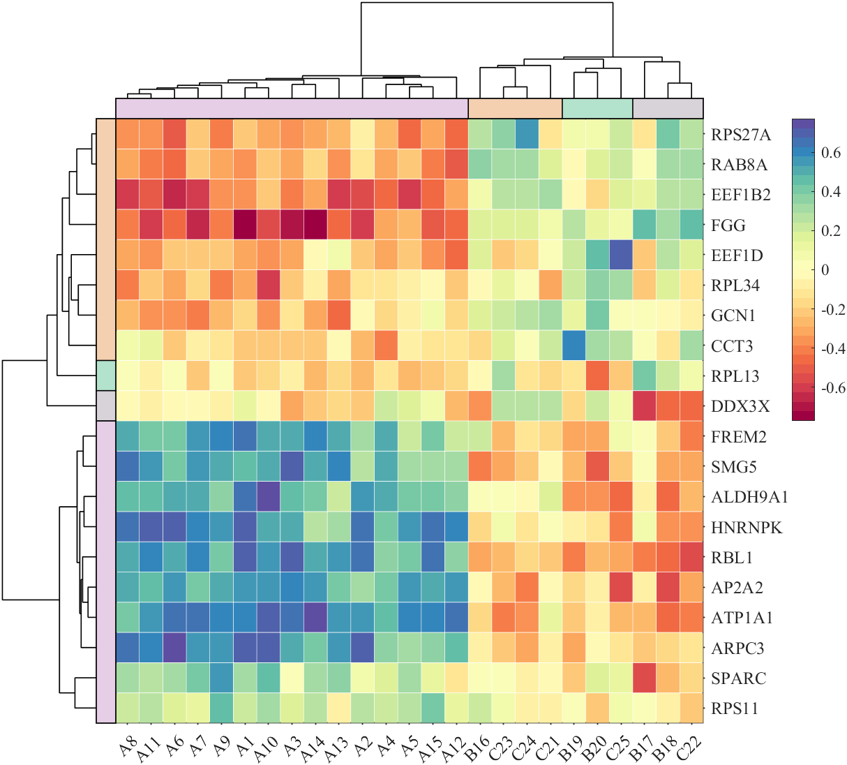
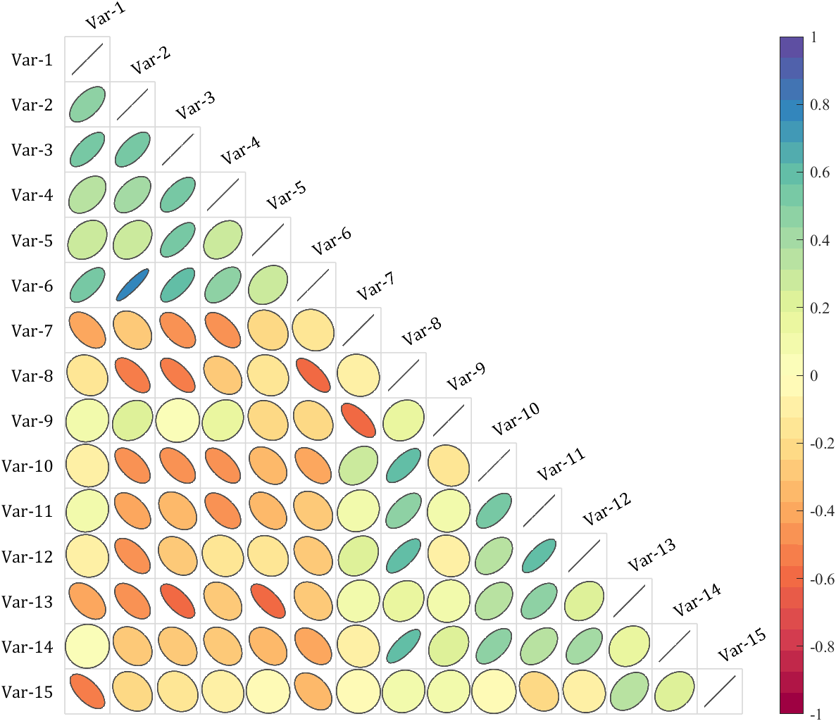
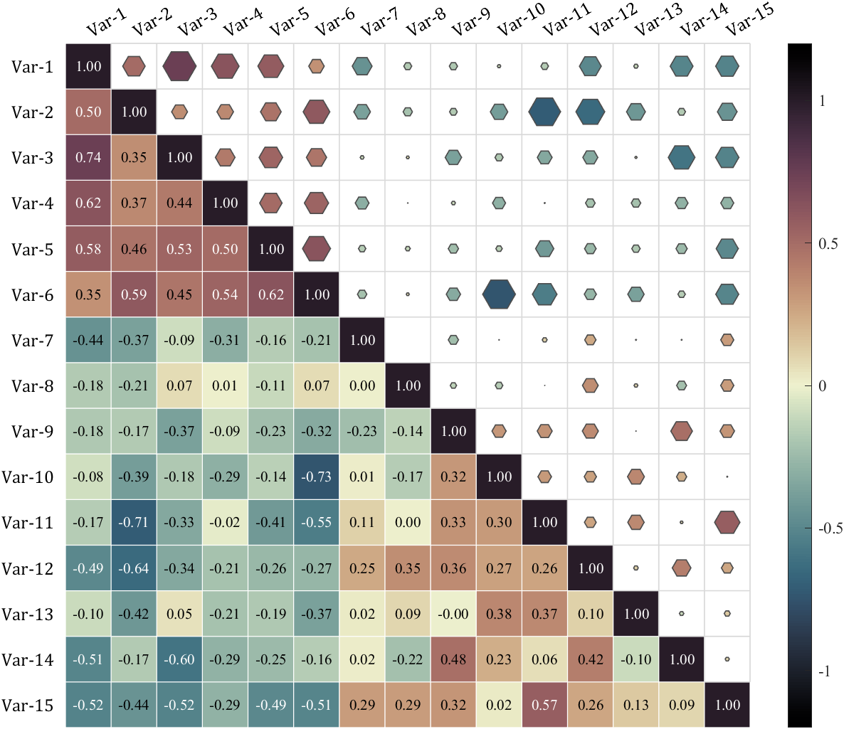
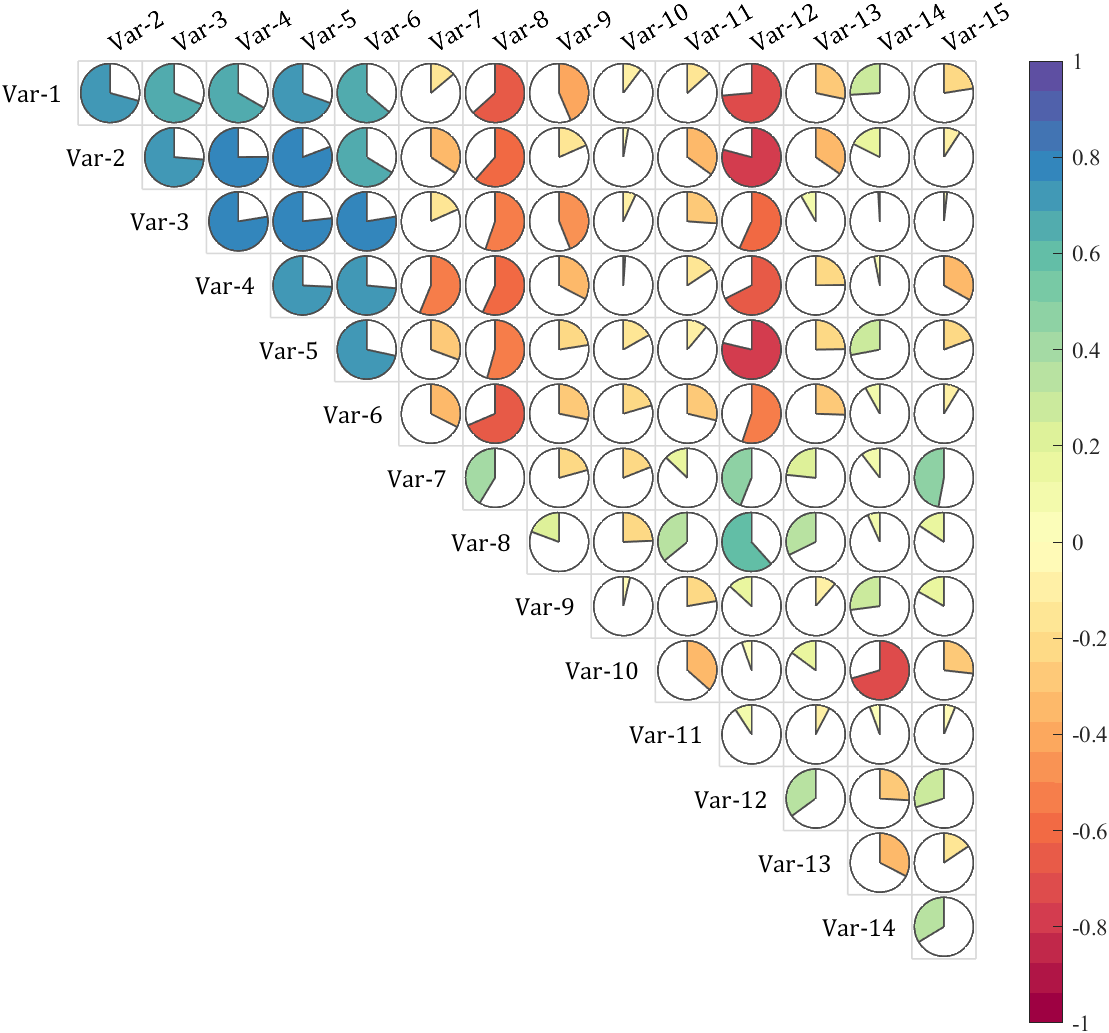
It is pretty easy to draw a cool heatmap for I have uploaded a tool to fileexchange:
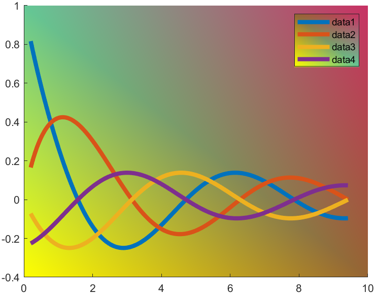
t=0.2:0.01:3*pi;
hold on
plot(t,cos(t)./(1+t),'LineWidth',4)
plot(t,sin(t)./(1+t),'LineWidth',4)
plot(t,cos(t+pi/2)./(1+t+pi/2),'LineWidth',4)
plot(t,cos(t+pi)./(1+t+pi),'LineWidth',4)
ax=gca;
hLegend=legend();
pause(1e-16)
colorData = uint8([255, 150, 200, 100; ...
255, 100, 50, 200; ...
0, 50, 100, 150; ...
102, 150, 200, 50]);
set(ax.Backdrop.Face, 'ColorBinding','interpolated','ColorData',colorData);
set(hLegend.BoxFace,'ColorBinding','interpolated','ColorData',colorData)
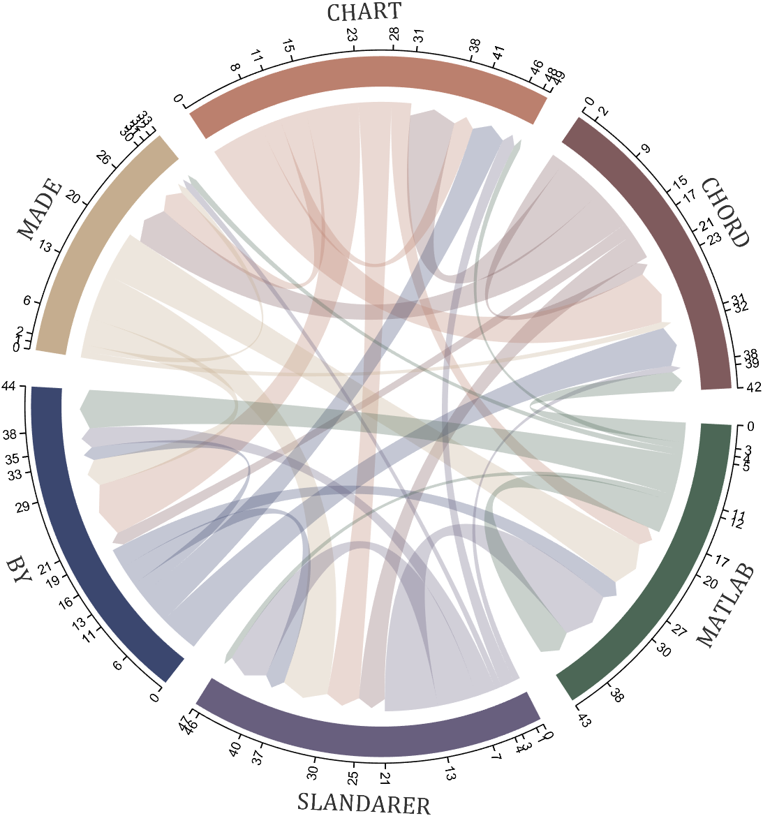
I have written two tools and uploaded fileexchange, which allows us to easily draw chord diagrams:
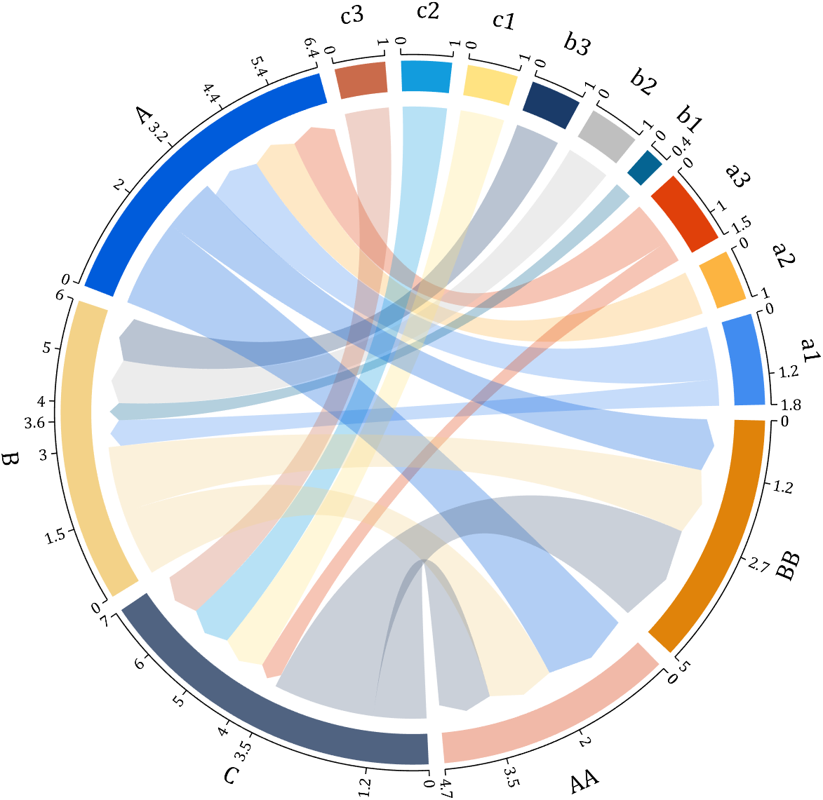

chord chart 弦图
download:
demo:
dataMat=[2 0 1 2 5 1 2;
3 5 1 4 2 0 1;
4 0 5 5 2 4 3];
dataMat=dataMat+rand(3,7);
dataMat(dataMat<1)=0;
colName={'G1','G2','G3','G4','G5','G6','G7'};
rowName={'S1','S2','S3'};
CC=chordChart(dataMat,'rowName',rowName,'colName',colName);
CC=CC.draw();
CC.setFont('FontSize',17,'FontName','Cambria')
% 显示刻度和数值
% Displays scales and numeric values
CC.tickState('on')
CC.tickLabelState('on')
% 调节标签半径
% Adjustable Label radius
CC.setLabelRadius(1.4);

Digraph chord chart 有向弦图
download:
demo:
dataMat=randi([0,8],[6,6]);
% 添加标签名称
NameList={'CHORD','CHART','MADE','BY','SLANDARER','MATLAB'};
BCC=biChordChart(dataMat,'Label',NameList,'Arrow','on');
BCC=BCC.draw();
% 添加刻度
BCC.tickState('on')
% 修改字体,字号及颜色
BCC.setFont('FontName','Cambria','FontSize',17,'Color',[.2,.2,.2])
BCC.setLabelRadius(1.3);
BCC.tickLabelState('on')
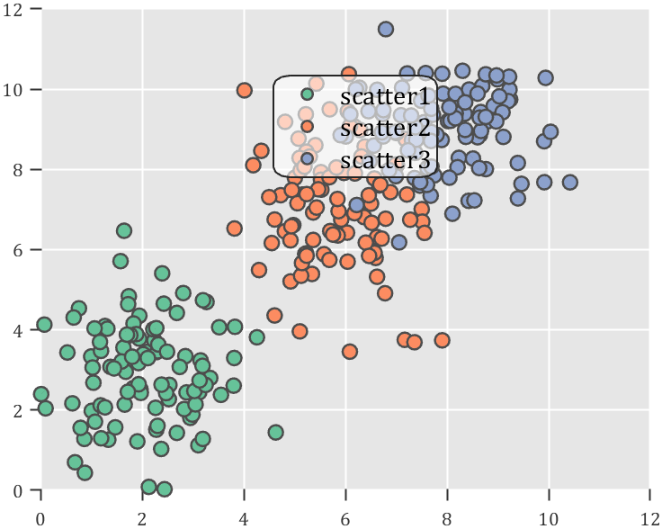
How to create a legend as follows?

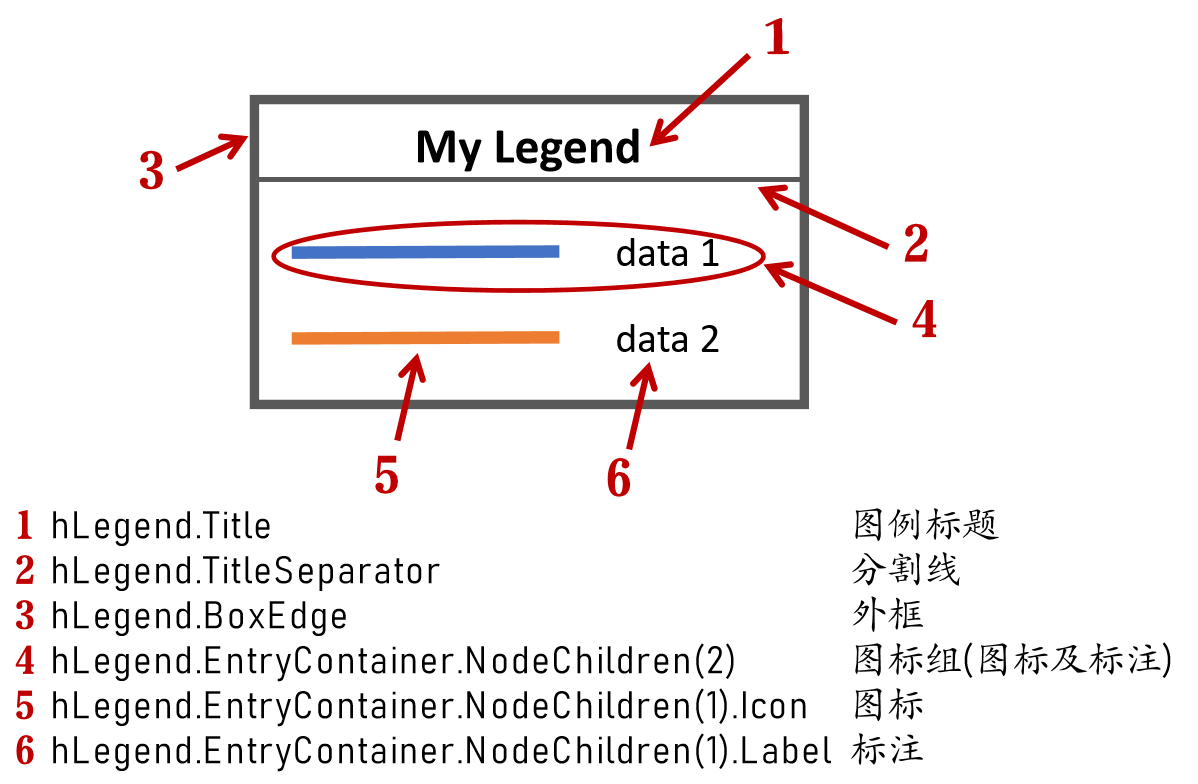
Principle Explanation - Graphic Objects
Hidden Properties of Legend are laid as follows
In most cases, legends are drawn using LineLoop and Quadrilateral:
Both of these basic graphic objects are drawn in groups of four points, and the general principle is as follows:

Of course, you can arrange the points in order, or set VertexIndices whitch means the vertex order to obtain the desired quadrilateral shape:

Other objects
Compared to objects that can only be grouped into four points, we also need to introduce more flexible objects. Firstly, LineStrip, a graphical object that draws lines in groups of two points:
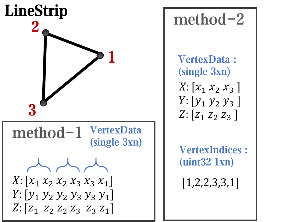
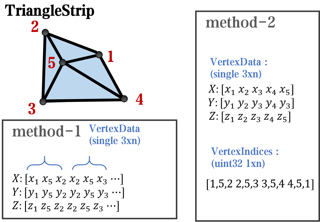
And TriangleStrip is a set of three points that draw objects to fill triangles, for example, complex polygons can be filled with multiple triangles:
Principle Explanation - Create and Replace
Let's talk about how to construct basic graphic objects, which are all constructed using undisclosed and very low-level functions, such as LineStrip, not through:
- LineStrip()
It is built through:
- matlab.graphics.primitive.world.LineStrip()
After building the object, the following properties must be set to make the hidden object visible:
- Layer
- ColorBinding
- ColorData
- VertexData
- PickableParts
The settings of these properties can refer to the original legend to form the object, which will not be elaborated here. You can also refer to the code I wrote.
Afterwards, set the newly constructed object's parent class as the Group parent class of the original component, and then hide the original component
newBoxEdgeHdl.Parent=oriBoxEdgeHdl.Parent;
oriBoxEdgeHdl.Visible='off';
The above is the entire process of component replacement, with two example codes written:
Semi transparent legend
function SPrettyLegend(lgd)
% Semitransparent rounded rectangle legend
% Copyright (c) 2023, Zhaoxu Liu / slandarer
% -------------------------------------------------------------------------
% Zhaoxu Liu / slandarer (2023). pretty legend
% (https://www.mathworks.com/matlabcentral/fileexchange/132128-pretty-legend),
% MATLAB Central File Exchange. 检索来源 2023/7/9.
% =========================================================================
if nargin<1
ax = gca;
lgd = get(ax,'Legend');
end
pause(1e-6)
Ratio = .1;
t1 = linspace(0,pi/2,4); t1 = t1([1,2,2,3,3,4]);
t2 = linspace(pi/2,pi,4); t2 = t2([1,2,2,3,3,4]);
t3 = linspace(pi,3*pi/2,4); t3 = t3([1,2,2,3,3,4]);
t4 = linspace(3*pi/2,2*pi,4); t4 = t4([1,2,2,3,3,4]);
XX = [1,1,1-Ratio+cos(t1).*Ratio,1-Ratio,Ratio,Ratio+cos(t2).*Ratio,...
0,0,Ratio+cos(t3).*Ratio,Ratio,1-Ratio,1-Ratio+cos(t4).*Ratio];
YY = [Ratio,1-Ratio,1-Ratio+sin(t1).*Ratio,1,1,1-Ratio+sin(t2).*Ratio,...
1-Ratio,Ratio,Ratio+sin(t3).*Ratio,0,0,Ratio+sin(t4).*Ratio];
% 圆角边框(border-radius)
oriBoxEdgeHdl = lgd.BoxEdge;
newBoxEdgeHdl = matlab.graphics.primitive.world.LineStrip();
newBoxEdgeHdl.AlignVertexCenters = 'off';
newBoxEdgeHdl.Layer = 'front';
newBoxEdgeHdl.ColorBinding = 'object';
newBoxEdgeHdl.LineWidth = 1;
newBoxEdgeHdl.LineJoin = 'miter';
newBoxEdgeHdl.WideLineRenderingHint = 'software';
newBoxEdgeHdl.ColorData = uint8([38;38;38;0]);
newBoxEdgeHdl.VertexData = single([XX;YY;XX.*0]);
newBoxEdgeHdl.Parent=oriBoxEdgeHdl.Parent;
oriBoxEdgeHdl.Visible='off';
% 半透明圆角背景(Semitransparent rounded background)
oriBoxFaceHdl = lgd.BoxFace;
newBoxFaceHdl = matlab.graphics.primitive.world.TriangleStrip();
Ind = [1:(length(XX)-1);ones(1,length(XX)-1).*(length(XX)+1);2:length(XX)];
Ind = Ind(:).';
newBoxFaceHdl.PickableParts = 'all';
newBoxFaceHdl.Layer = 'back';
newBoxFaceHdl.ColorBinding = 'object';
newBoxFaceHdl.ColorType = 'truecoloralpha';
newBoxFaceHdl.ColorData = uint8(255*[1;1;1;.6]);
newBoxFaceHdl.VertexData = single([XX,.5;YY,.5;XX.*0,0]);
newBoxFaceHdl.VertexIndices = uint32(Ind);
newBoxFaceHdl.Parent = oriBoxFaceHdl.Parent;
oriBoxFaceHdl.Visible = 'off';
end
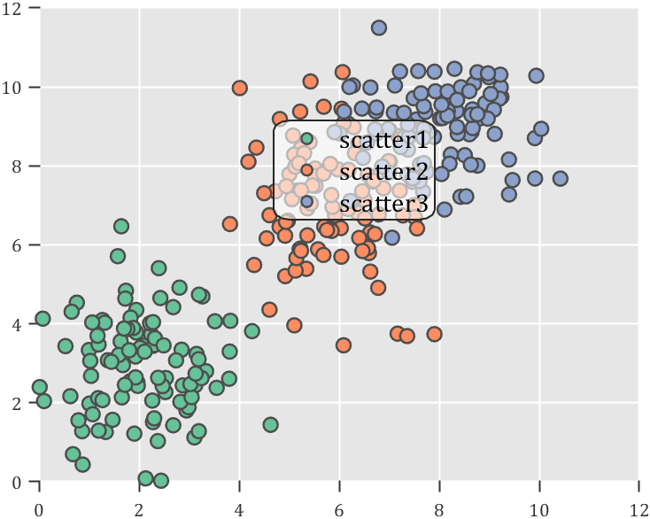
Usage examples
clc; clear; close all
rng(12)
% 生成随机点(Generate random points)
mu = [2 3; 6 7; 8 9];
S = cat(3,[1 0; 0 2],[1 0; 0 2],[1 0; 0 1]);
r1 = abs(mvnrnd(mu(1,:),S(:,:,1),100));
r2 = abs(mvnrnd(mu(2,:),S(:,:,2),100));
r3 = abs(mvnrnd(mu(3,:),S(:,:,3),100));
% 绘制散点图(Draw scatter chart)
hold on
propCell = {'LineWidth',1.2,'MarkerEdgeColor',[.3,.3,.3],'SizeData',60};
scatter(r1(:,1),r1(:,2),'filled','CData',[0.40 0.76 0.60],propCell{:});
scatter(r2(:,1),r2(:,2),'filled','CData',[0.99 0.55 0.38],propCell{:});
scatter(r3(:,1),r3(:,2),'filled','CData',[0.55 0.63 0.80],propCell{:});
% 增添图例(Draw legend)
lgd = legend('scatter1','scatter2','scatter3');
lgd.Location = 'northwest';
lgd.FontSize = 14;
% 坐标区域基础修饰(Axes basic decoration)
ax=gca; grid on
ax.FontName = 'Cambria';
ax.Color = [0.9,0.9,0.9];
ax.Box = 'off';
ax.TickDir = 'out';
ax.GridColor = [1 1 1];
ax.GridAlpha = 1;
ax.LineWidth = 1;
ax.XColor = [0.2,0.2,0.2];
ax.YColor = [0.2,0.2,0.2];
ax.TickLength = [0.015 0.025];
% 隐藏轴线(Hide XY-Ruler)
pause(1e-6)
ax.XRuler.Axle.LineStyle = 'none';
ax.YRuler.Axle.LineStyle = 'none';
SPrettyLegend(lgd)
Heart shaped legend (exclusive to pie charts)
function pie2HeartLegend(lgd)
% Heart shaped legend for pie chart
% Copyright (c) 2023, Zhaoxu Liu / slandarer
% -------------------------------------------------------------------------
% Zhaoxu Liu / slandarer (2023). pretty legend
% (https://www.mathworks.com/matlabcentral/fileexchange/132128-pretty-legend),
% MATLAB Central File Exchange. 检索来源 2023/7/9.
% =========================================================================
if nargin<1
ax = gca;
lgd = get(ax,'Legend');
end
pause(1e-6)
% 心形曲线(Heart curve)
x = -1:1/100:1;
y1 = 0.6 * abs(x) .^ 0.5 + ((1 - x .^ 2) / 2) .^ 0.5;
y2 = 0.6 * abs(x) .^ 0.5 - ((1 - x .^ 2) / 2) .^ 0.5;
XX = [x, flip(x),x(1)]./3.4+.5;
YY = ([y1, y2,y1(1)]-.2)./2+.5;
Ind = [1:(length(XX)-1);2:length(XX)];
Ind = Ind(:).';
% 获取图例图标(Get Legend Icon)
lgdEntryChild = lgd.EntryContainer.NodeChildren;
iconSet = arrayfun(@(lgdEntryChild)lgdEntryChild.Icon.Transform.Children.Children,lgdEntryChild,UniformOutput=false);
% 基础边框句柄(Base Border Handle)
newEdgeHdl = matlab.graphics.primitive.world.LineStrip();
newEdgeHdl.AlignVertexCenters = 'off';
newEdgeHdl.Layer = 'front';
newEdgeHdl.ColorBinding = 'object';
newEdgeHdl.LineWidth = .8;
newEdgeHdl.LineJoin = 'miter';
newEdgeHdl.WideLineRenderingHint = 'software';
newEdgeHdl.ColorData = uint8([38;38;38;0]);
newEdgeHdl.VertexData = single([XX;YY;XX.*0]);
newEdgeHdl.VertexIndices = uint32(Ind);
% 基础多边形面句柄(Base Patch Handle)
newFaceHdl = matlab.graphics.primitive.world.TriangleStrip();
Ind = [1:(length(XX)-1);ones(1,length(XX)-1).*(length(XX)+1);2:length(XX)];
Ind = Ind(:).';
newFaceHdl.PickableParts = 'all';
newFaceHdl.Layer = 'middle';
newFaceHdl.ColorBinding = 'object';
newFaceHdl.ColorType = 'truecoloralpha';
newFaceHdl.ColorData = uint8(255*[1;1;1;.6]);
newFaceHdl.VertexData = single([XX,.5;YY,.5;XX.*0,0]);
newFaceHdl.VertexIndices = uint32(Ind);
% 替换图例图标(Replace Legend Icon)
for i = 1:length(iconSet)
oriEdgeHdl = iconSet{i}(1);
tNewEdgeHdl = copy(newEdgeHdl);
tNewEdgeHdl.ColorData = oriEdgeHdl.ColorData;
tNewEdgeHdl.Parent = oriEdgeHdl.Parent;
oriEdgeHdl.Visible = 'off';
oriFaceHdl = iconSet{i}(2);
tNewFaceHdl = copy(newFaceHdl);
tNewFaceHdl.ColorData = oriFaceHdl.ColorData;
tNewFaceHdl.Parent = oriFaceHdl.Parent;
oriFaceHdl.Visible = 'off';
end
end
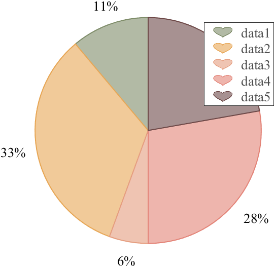
Usage examples
clc; clear; close all
% 生成随机点(Generate random points)
X = [1 3 0.5 2.5 2];
pieHdl = pie(X);
% 修饰饼状图(Decorate pie chart)
colorList=[0.4941 0.5490 0.4118
0.9059 0.6510 0.3333
0.8980 0.6157 0.4980
0.8902 0.5137 0.4667
0.4275 0.2824 0.2784];
for i = 1:2:length(pieHdl)
pieHdl(i).FaceColor=colorList((i+1)/2,:);
pieHdl(i).EdgeColor=colorList((i+1)/2,:);
pieHdl(i).LineWidth=1;
pieHdl(i).FaceAlpha=.6;
end
for i = 2:2:length(pieHdl)
pieHdl(i).FontSize=13;
pieHdl(i).FontName='Times New Roman';
end
lgd=legend('FontSize',13,'FontName','Times New Roman','TextColor',[1,1,1].*.3);
pie2HeartLegend(lgd)
I found this list on Book Authority about the top MATLAB books: https://bookauthority.org/books/best-matlab-books
My favorite book is Accelerating MATLAB Performance - 1001 tips to speed up MATLAB programs. I always pick something up from the book that helps me out.
A key aspect to masting MATLAB Graphics is getting a hang of the MATLAB Graphics Object Hierarchy which is essentially the structure of MATLAB figures that is used in the rendering pipeline. The base object is the Graphics Root (see groot) which contains the Figure. The Figure contains Axes or other containers such as a Tiled Chart Layout (see tiledlayout). Then these Axes can contain graphics primatives (the objects that contain data and get rendered) such as Lines or Patches.
Every graphics object has two important properties, the "Parent" and "Children" properties which can be used to access other objects in the tree. This can be very useful when trying to customize a pre-built chart (such as adding grid lines to both axes in an eye diagram chart) or when trying to access the axes of a non-current figure via a primative (so "gca" doesn't help out).
One last Tip and Trick with this is that you can declare graphics primatives without putting them on or creating an Axes by setting the first input argument to "gobjects(0)" which is an empty array of placeholder graphics objects. Then, when you have an Axes to plot the primitive on and are ready to render it, you can set the "Parent" of the object to your new Axes.
For Example:
l = line(gobjects(0), 1:10, 1:10);
...
...
...
l.Parent = gca;
Practicing navigating and exploring this tree will help propel your understanding of plotting in MATLAB.
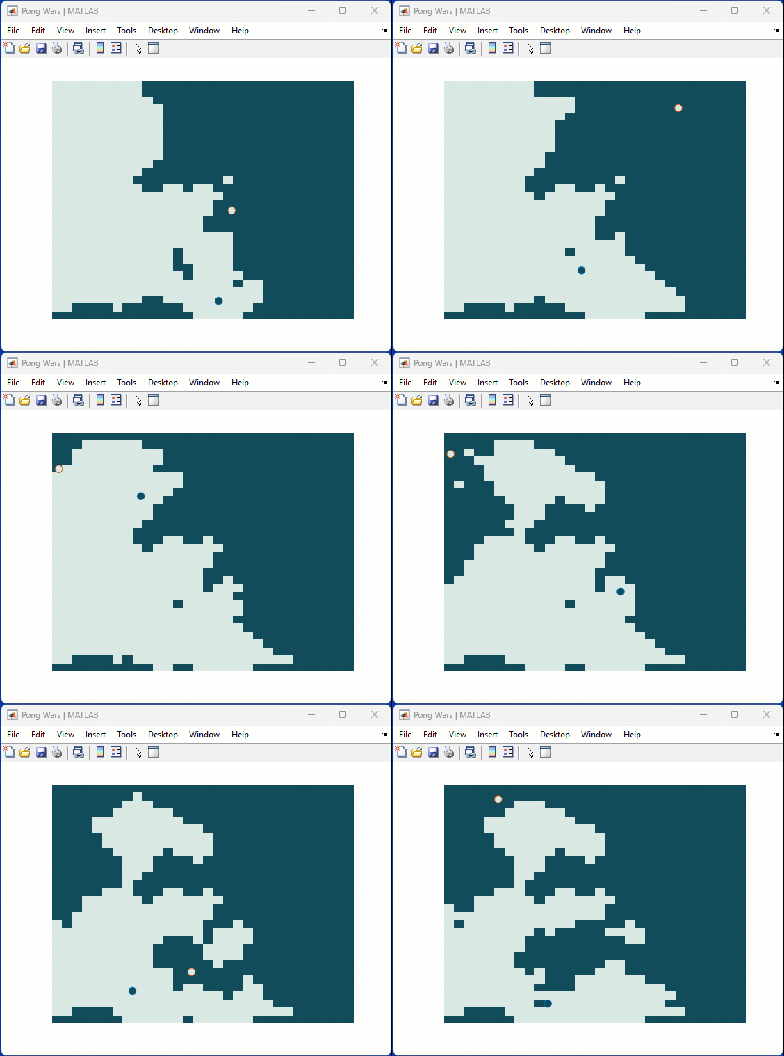
One of my colleauges, Michio, recently posted an implementation of Pong Wars in MATLAB
- Here's the code on GitHub.https://lnkd.in/gZG-AsFX
- If you want to open with MATLAB Online, click here https://lnkd.in/gahrTMW5
- He saw this first here: https://lnkd.in/gu_Z-Pks
Making me wonder about variations. What might the resulting patterns look with differing numbers of balls? Different physics etc?
spy
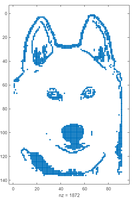
Over at Reddit, a MATLAB user asked about when to use a script vs. a live script. How would you answer this?
Starting with MATLAB can be daunting, but the right resources make all the difference. In my experience, the combination of MATLAB Onramp and Cody offers an engaging start.
MATLAB Onramp introduces you to MATLAB's basic features and workflows. Then practice your coding skill on Cody. Challenge yourself to solve 1 basic problem every day for a month! This consistent practice can significantly enhance your proficiency.
What other resources have helped you on your MATLAB journey? Share your recommendations and let's create a comprehensive learning path for beginners!
I would tell myself to understand vectorization. MATLAB is designed for operating on whole arrays and matrices at once. This is often more efficient than using loops.
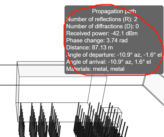
how can I do to get those informations?
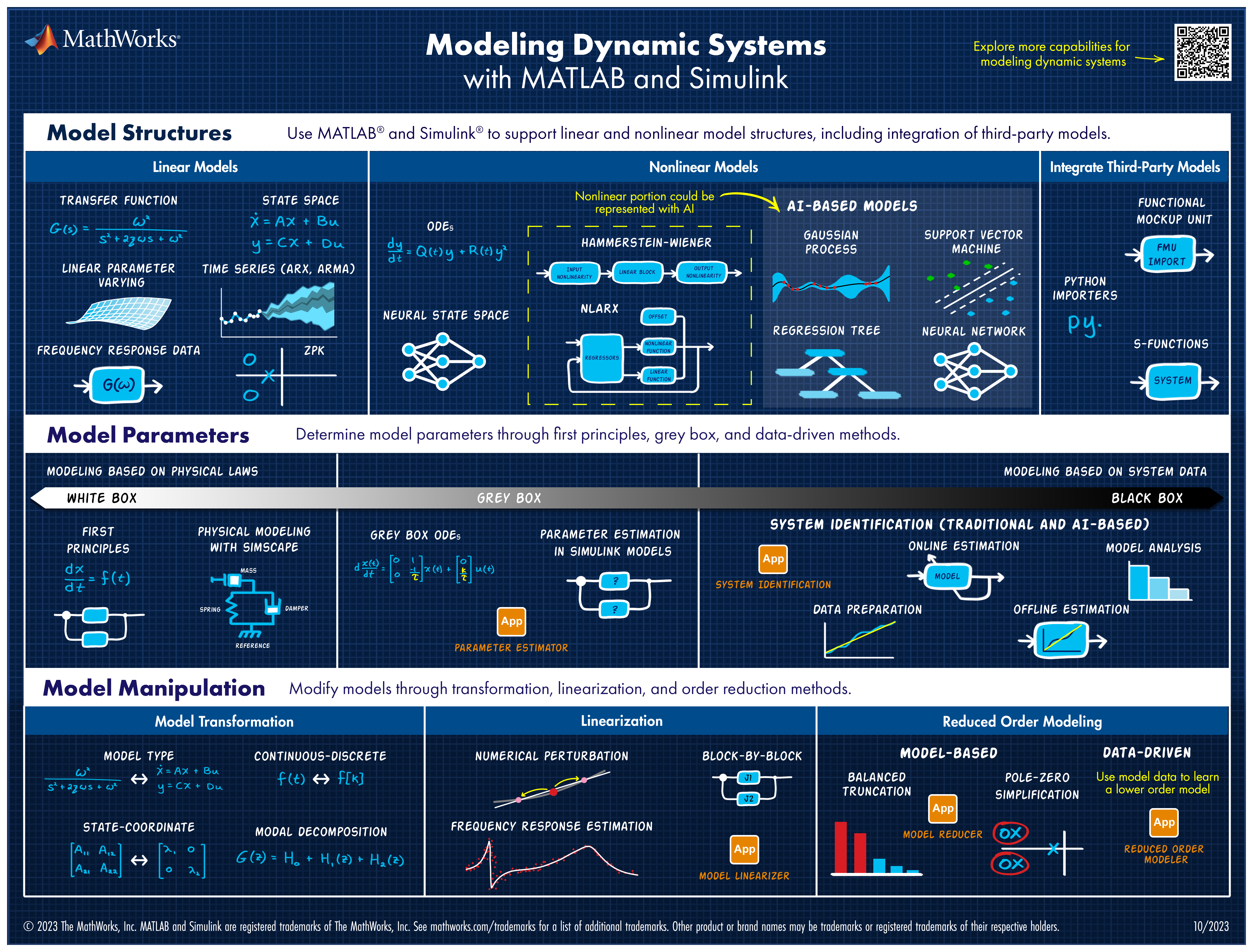
Explore all the capabilities for Modeling Dynamic Systems while keeping them handy with this Cheat Sheet - Download Now.
We are thrilled to announce the grand prize winners of our MATLAB Flipbook contest! This year, we invited the MATLAB Graphics Infrastructure team, renowned for their expertise in exporting and animation workflows, to be our judges. After careful consideration, they have selected the top three winners:
Judge comments: Creative and realistic rendering with well-written code
2nd place - Christmas Tree / Zhaoxu Liu
Judge comments: Festive and advanced animation that is appropriate to the current holiday season.
Judge comments: Nice translation of existing shader logic to MATLAB that produces an advanced and appealing visual effect.
In addition, after validating the votes, we are pleased to announce the top 10 participants on the leaderboard:
- Tim
- Zhaoxu Liu / slandarer
- KARUPPASAMYPANDIYAN M
- Dhimas Mahardika S.Si., M.Mat
- Augusto Mazzei
- Jenny Bosten
- Lucas
- Jr
- Victoria
- ME
Congratulations to all! Your creativity and skills have inspired many of us to explore and learn new skills, and make this contest a big success!
The MATLAB Flipbook Mini Hack contest has concluded! During the 4 weeks, over 600 creative animations have been created. We had a lot of fun and a great learning experience! Thank you, everyone!
Now it’s the time to announce week 4 winners. Note that grand prize winners will be announced shortly after we validate votes on winning entries.
Realism:
Holiday & Season:
Abstract:
Cartoon:
Congratulations, weekly winners!We will reach out to you shortly for your prizes.
Looking for an opportunity to practice your AI skills on a real-world problem? Interested in AI for climage change? Sign up for the Kelp Wanted challenge, which tasks participants with developing an algorithm that can detect the presence of kelp forests from satellite images.
Participants of all skill levels from anywhere in the world are welcome to compete!
MathWorks provides the following resources for all participants:
Have you marveled at the breathtaking, natural-looking animations crafted by the creative minds in the Flipbook Mini Hack contest? Think of @Tim, @Jenny Bosten, and @Zhaoxu Liu / slandarer- their work is nothing short of extraordinary.

So, what's their secret? Adam Danz, a developer in the MATLAB Graphics and Charting team and a top community contributor, has graciously unveiled the mysteries in his latest blog post - "Creating natural textures with power-law noise: clouds, terrains, and more." The post offers simple, step-by-step instructions and code snippets, empowering you to grasp these enchanting techniques effortlessly.
Check it out and we hope it sparks your creativity and serves as a wellspring of inspiration. With only 3 days remaining before the contest draws to a close, it's time to dive into the code and let your imagination soar!
In Week 3, we reached the 400-animations milestone! Let’s work together to achieve the 500-animations goal!
During the last week of the contest, we strongly encourage you to inspire your colleagues, classmates, or friends to vote. Voters will also have the opportunity to win a MATLAB T-shirt.
Mini Hack Winners - Week 3
Math, Physics, or Science explanation:
Most creative remix:
40:
Math is beautiful:
Mashup (Combined themes):
Nature:
Holidays:
Congratulations, winners!
In week 4, we’d love to see more entries in the following categories:
- Holidays:
- Seasons:
- Abstract:
- Mashup (mixed categories)
A gentle reminder that you have a direct impact on the next generation of animation tools in MATLAB! Don’t forget to share your thoughts and ideas with us.

