主要内容
Results for
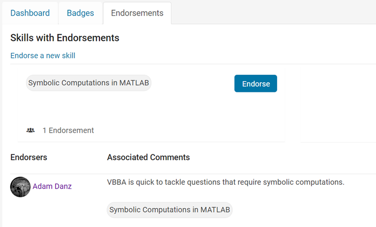
Big congratulations to @VBBV for achieving the remarkable milestone of 3,000 reputation points, earning the prestigious title of Editor within our community.
This achievement is a testament to @VBBV's exceptional contributions and steadfast commitment to the community. These efforts have also been endorsed by fellow top contributors, underscoring the value and impact of @VBBV's expertise.
Welcome to the Editors' Club, @VBBV – we are excited to witness and support your continued journey and influence within our community!
eye(3) - diag(ones(1,3))
11%
0 ./ ones(3)
9%
cos(repmat(pi/2, [3,3]))
16%
zeros(3)
20%
A(3, 3) = 0
32%
mtimes([1;1;0], [0,0,0])
12%
3009 个投票
MATLAB O/X Quiz
Answer BEFORE Googling!
- An infinite loop can be made using "for".
- "A == A" is always true.
- "round(2.5)" is 3.
- "round(-0.5)" is 0.
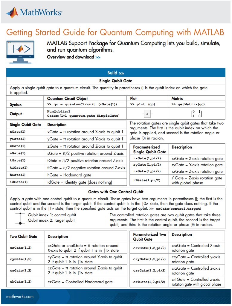
MATLAB Support Package for Quantum Computing lets you build, simulate, and run quantum algorithms.
Check out the Cheat Sheet here!
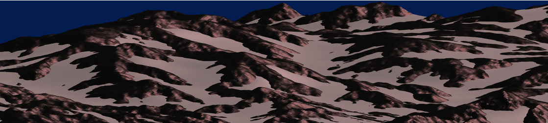
I think that MATLAB's Flipbook Mini Hack had quite some inspiring entries. My work largely deals with digital elevation models (DEMs). Hence I really liked the random renderings of landscapes, in particular this one written by Tim which inspired me to adopt the code and apply to the example data that comes with my software TopoToolbox. The results and code are shown here.
and immeditaely everyone wanted the code! It turns out that this is the result of my remix of @Zhaoxu Liu / slandarer's entry on the MATLAB Flipbook Mini Hack.
I pointed people to the Flipbook entry but, of course, that just gave the code to render a single frame and people wanted the full code to render the animated gif. That way, they could make personalised versions
I just published a blog post that gives the code used by the team behind the Mini Hack to produce the animated .gifs https://blogs.mathworks.com/matlab/2024/02/16/producing-animated-gifs-from-matlab-flipbook-mini-hack-entries/
Thanks again to @Zhaoxu Liu / slandarer for a great entry that seems like it will live for a long time :)
If you've dabbled in "procedural generation," (algorithmically generating natural features), you may have come across the problem of sphere texturing. How to seamlessly texture a sphere is not immediately obvious. Watch what happens, for example, if you try adding power law noise to an evenly sampled grid of spherical angle coordinates (i.e. a "UV sphere" in Blender-speak):
% Example: how [not] to texture a sphere:
rng(2, 'twister'); % Make what I have here repeatable for you
% Make our radial noise, mapped onto an equal spaced longitude and latitude
% grid.
N = 51;
b = linspace(-1, 1, N).^2;
r = abs(ifft2(exp(6i*rand(N))./(b'+b+1e-5))); % Power law noise
r = rescale(r, 0, 1) + 5;
[lon, lat] = meshgrid(linspace(0, 2*pi, N), linspace(-pi/2, pi/2, N));
[x2, y2, z2] = sph2cart(lon, lat, r);
r2d = @(x)x*180/pi;
% Radial surface texture
subplot(1, 3, 1);
imagesc(r, 'Xdata', r2d(lon(1,:)), 'Ydata', r2d(lat(:, 1)));
xlabel('Longitude (Deg)');
ylabel('Latitude (Deg)');
title('Texture (radial variation)');
% View from z axis
subplot(1, 3, 2);
surf(x2, y2, z2, r);
axis equal
view([0, 90]);
title('Top view');
% Side view
subplot(1, 3, 3);
surf(x2, y2, z2, r);
axis equal
view([-90, 0]);
title('Side view');
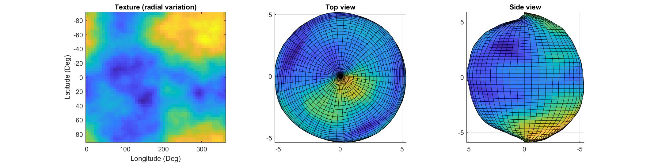
The created surface shows "pinching" at the poles due to different radial values mapping to the same location. Furthermore, the noise statistics change based on the density of the sampling on the surface.
How can this be avoided? One standard method is to create a textured volume and sample the volume at points on a sphere. Code for doing this is quite simple:
rng default % Make our noise realization repeatable
% Create our 3D power-law noise
N = 201;
b = linspace(-1, 1, N);
[x3, y3, z3] = meshgrid(b, b, b);
b3 = x3.^2 + y3.^2 + z3.^2;
r = abs(ifftn(ifftshift(exp(6i*randn(size(b3)))./(b3.^1.2 + 1e-6))));
% Modify it - make it more interesting
r = rescale(r);
r = r./(abs(r - 0.5) + .1);
% Sample on a sphere
[x, y, z] = sphere(500);
% Plot
ir = interp3(x3, y3, z3, r, x, y, z, 'linear', 0);
surf(x, y, z, ir);
shading flat
axis equal off
set(gcf, 'color', 'k');
colormap(gray);
The result of evaluating this code is a seamless, textured sphere with no discontinuities at the poles or variation in the spatial statistics of the noise texture:
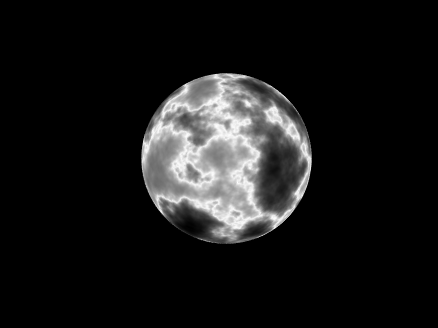
But what if you want to smooth it or perform some other local texture modification? Smoothing the volume and resampling is not equivalent to smoothing the surficial features shown on the map above.
A more flexible alternative is to treat the samples on the sphere surface as a set of interconnected nodes that are influenced by adjacent values. Using this approach we can start by defining the set of nodes on a sphere surface. These can be sampled almost arbitrarily, though the noise statistics will vary depending on the sampling strategy.
One noise realisation I find attractive can be had by randomly sampling a sphere. Normalizing a point in N-dimensional space by its 2-norm projects it to the surface of an N-dimensional unit sphere, so randomly sampling a sphere can be done very easily using randn() and vecnorm():
N = 5e3; % Number of nodes on our sphere
g=randn(3,N); % Random 3D points around origin
p=g./vecnorm(g); % Projected to unit sphere
The next step is to find each point's "neighbors." The first step is to find the convex hull. Since each point is on the sphere, the convex hull will include each point as a vertex in the triangulation:
k=convhull(p');
In the above, k is an N x 3 set of indices where each row represents a unique triangle formed by a triplicate of points on the sphere surface. The vertices of the full set of triangles containing a point describe the list of neighbors to that point.
What we want now is a large, sparse symmetric matrix where the indices of the columns & rows represent the indices of the points on the sphere and the nth row (and/or column) contains non-zero entries at the indices corresponding to the neighbors of the nth point.
How to do this? You could set up a tiresome nested for-loop searching for all rows (triangles) in k that contain some index n, or you could directly index via:
c=@(x)sparse(k(:,x)*[1,1,1],k,1,N,N);
t=c(1)|c(2)|c(3);
The result is the desired sparse connectivity matrix: a matrix with non-zero entries defining neighboring points.
So how do we create a textured sphere with this connectivity matrix? We will use it to form a set of equations that, when combined with the concept of "regularization," will allow us to determine the properties of the randomness on the surface. Our regularizer will penalize the difference of the radial distance of a point and the average of its neighbors. To do this we replace the main diagonal with the negative of the sum of the off-diagonal components so that the rows and columns are zero-mean. This can be done via:
w=spdiags(-sum(t,2)+1,0,double(t));
Now we invoke a bit of linear algebra. Pretend x is an N-length vector representing the radial distance of each point on our sphere with the noise realization we desire. Y will be an N-length vector of "observations" we are going to generate randomly, in this case using a uniform distribution (because it has a bias and we want a non-zero average radius, but you can play around with different distributions than uniform to get different effects):
Y=rand(N,1);
and A is going to be our "transformation" matrix mapping x to our noisy observations:
Ax = Y
In this case both x and Y are N length vectors and A is just the identity matrix:
A = speye(N);
Y, however, doesn't create the noise realization we want. So in the equation above, when solving for x we are going to introduce a regularizer which is going to penalize unwanted behavior of x by some amount. That behavior is defined by the point-neighbor radial differences represented in matrix w. Our estimate of x can then be found using one of my favorite Matlab assets, the "\" operator:
smoothness = 10; % Smoothness penalty: higher is smoother
x = (A+smoothness*w'*w)\Y; % Solving for radii
The vector x now contains the radii with the specified noise realization for the sphere which can be created simply by multiplying x by p and plotting using trisurf:
p2 = p.*x';
trisurf(k,p2(1,:),p2(2,:),p2(3,:),'FaceC', 'w', 'EdgeC', 'none','AmbientS',0,'DiffuseS',0.6,'SpecularS',1);
light;
set(gca, 'color', 'k');
axis equal
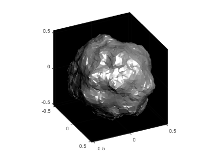
The following images show what happens as you change the smoothness parameter using values [.1, 1, 10, 100] (left to right):
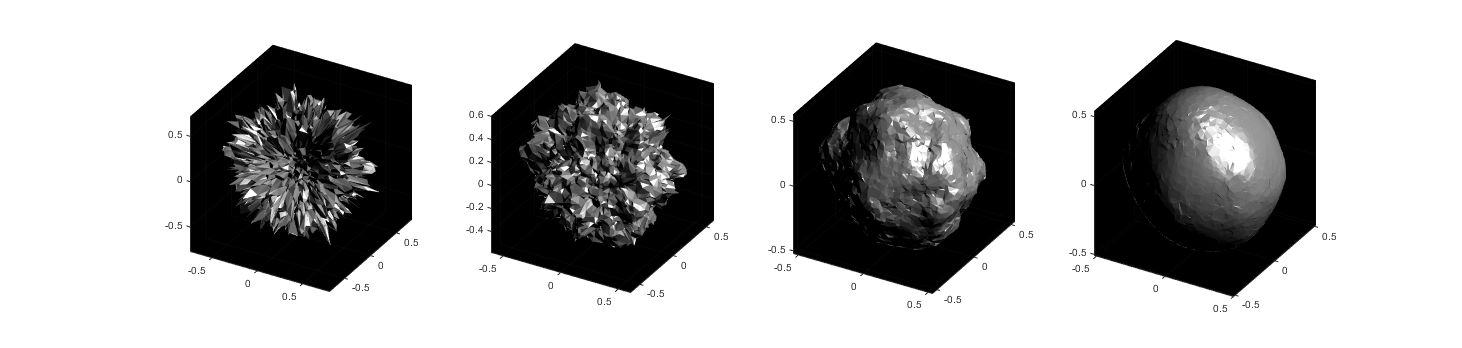
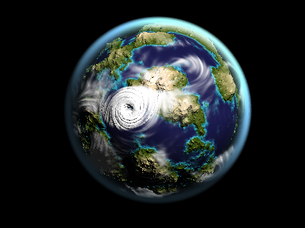
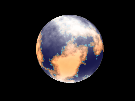
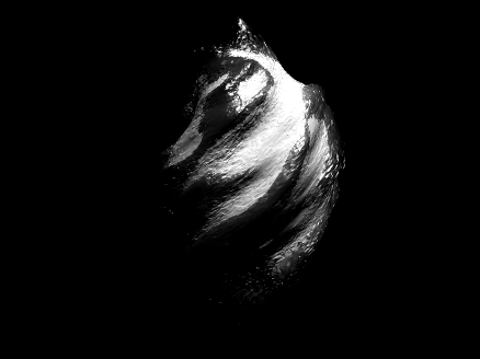
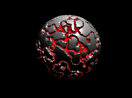
Now you know a couple ways to make a textured sphere: that's the starting point for having a lot of fun with basic procedural planet, moon, or astroid generation! Here's some examples of things you can create based on these general ideas:
The MATLAB command window isn't just for commands and outputs—it can also host interactive hyperlinks. These can serve as powerful shortcuts, enhancing the feedback you provide during code execution. Here are some hyperlinks I frequently use in fprintf statements, warnings, or error messages.
1. Open a website.
msg = "Could not download data from website.";
url = "https://blogs.mathworks.com/graphics-and-apps/";
hypertext = "Go to website"
fprintf(1,'%s <a href="matlab: web(''%s'') ">%s</a>\n',msg,url,hypertext);
Could not download data from website. Go to website
2. Open a folder in file explorer (Windows)
msg = "File saved to current directory.";
directory = cd();
hypertext = "[Open directory]";
fprintf(1,'%s <a href="matlab: winopen(''%s'') ">%s</a>\n',msg,directory,hypertext)
File saved to current directory. [Open directory]
3. Open a document (Windows)
msg = "Created database.csv.";
filepath = fullfile(cd,'database.csv');
hypertext = "[Open file]";
fprintf(1,'%s <a href="matlab: winopen(''%s'') ">%s</a>\n',msg,filepath,hypertext)
Created database.csv. [Open file]
4. Open an m-file and go to a specific line
msg = 'Go to';
file = 'streamline.m';
line = 51;
fprintf(1,'%s <a href="matlab: matlab.desktop.editor.openAndGoToLine(which(''%s''), %d); ">%s line %d</a>', msg, file, line, file, line);
Go to streamline.m line 51
5. Display more text
msg = 'Incomplete data detected.';
extendedInfo = '\tFilename: m32c4r28\n\tDate: 12/20/2014\n\tElectrode: (3,7)\n\tDepth: ???\n';
hypertext = '[Click for more info]';
warning('%s <a href="matlab: fprintf(''%s'') ">%s</a>', msg,extendedInfo,hypertext);
<click>
- Filename: m32c4r28
- Date: 12/20/2014
- Electrode: (3,7)
- Depth: ???
6. Run a function
Similarly, you can also add hyperlinks in figures and apps
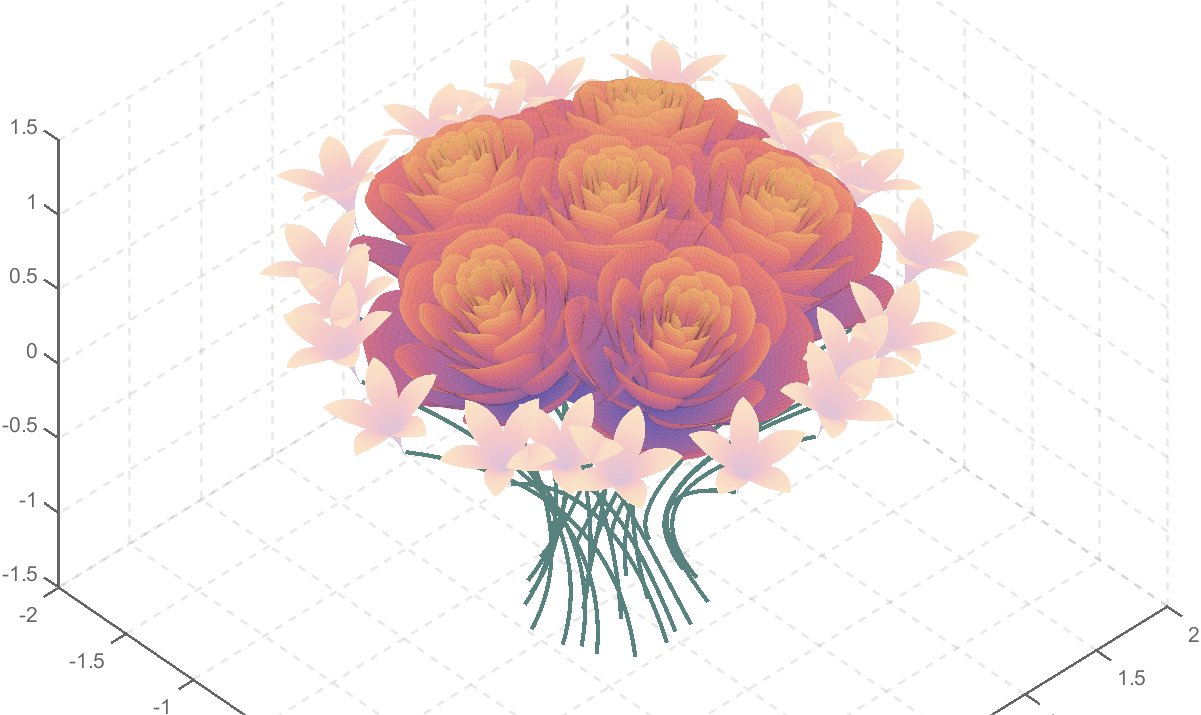
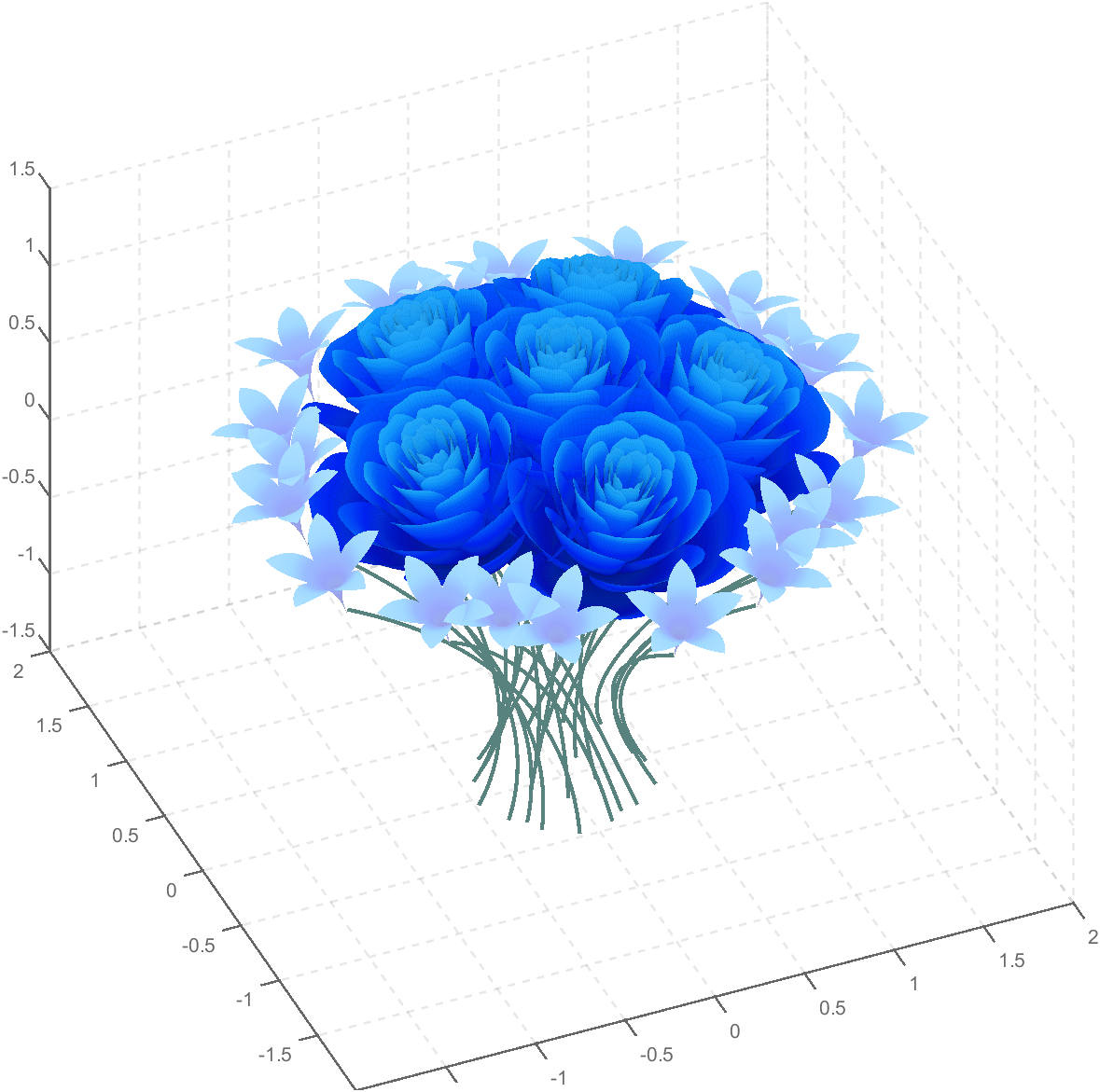
And what do you do for Valentine's Day?
which technical support should I contact/ask for the published Simscape example?
Happy year of the dragon.
To enlarge an array with more rows and/or columns, you can set the lower right index to zero. This will pad the matrix with zeros.
m = rand(2, 3) % Initial matrix is 2 rows by 3 columns
mCopy = m;
% Now make it 2 rows by 5 columns
m(2, 5) = 0
m = mCopy; % Go back to original matrix.
% Now make it 3 rows by 3 columns
m(3, 3) = 0
m = mCopy; % Go back to original matrix.
% Now make it 3 rows by 7 columns
m(3, 7) = 0
Greetings to all MATLAB users,
Although the MATLAB Flipbook contest has concluded, the pursuit of ‘learning while having fun’ continues. I would like to take this opportunity to highlight some recent insightful technical articles from a standout contest participant – Zhaoxu Liu / slandarer.
Zhaoxu has contributed eight informative articles to both the Tips & Tricks and Fun channels in our new Discussions area. His articles offer practical advice on topics such as customizing legends, constructing chord charts, and adding color to axes. Additionally, he has shared engaging content, like using MATLAB to create an interactive dragon that follows your mouse cursor, a nod to the upcoming Year of the Dragon in 2024!
I invite you to explore these articles for both enjoyment and education, and I hope you'll find new techniques to incorporate into your work.
Our community is full of individuals skilled in MATLAB, and we're always eager to learn from one another. Who would you like to see featured next? Or perhaps you have some tips & tricks of your own to contribute. Remember, sharing knowledge is a collaborative effort, as Confucius wisely stated, 'When I walk along with two others, they may serve me as my teachers.'
Let's maintain our commitment to a continuous learning journey. This could be the perfect warm-up for the upcoming 2024 contest.
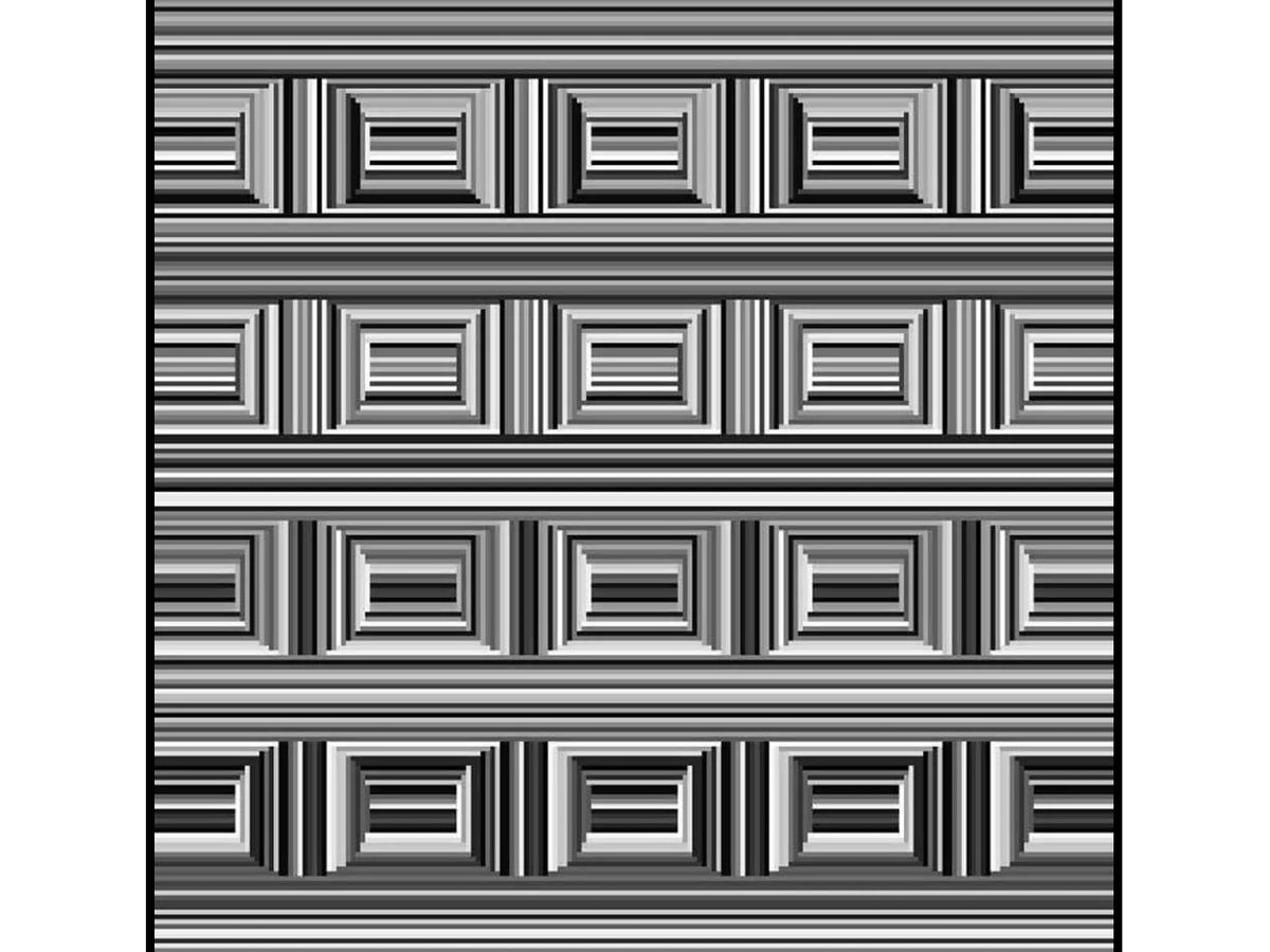
Can you see them?
I have been procrastinating on schoolwork by looking at all the amazing designs created in the last MATLAB Flipbook Mini Hack! They are just amazing. The voting is over but what are y'all's personal favorites? Mine is the flapping butterfly, it is for sure a creation I plan to share with others in the future!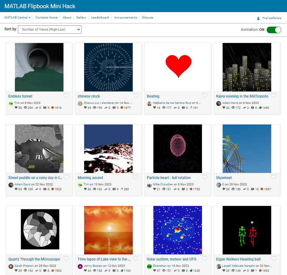
It is easy to obtain sankey plot like that using my tool:
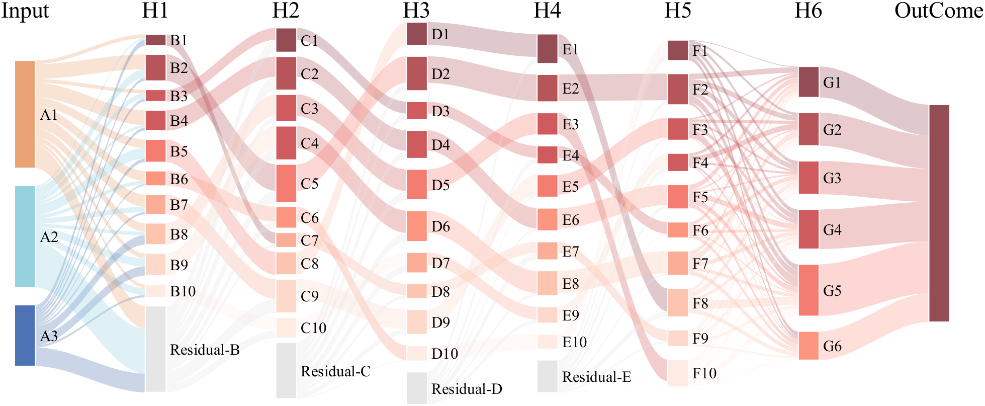
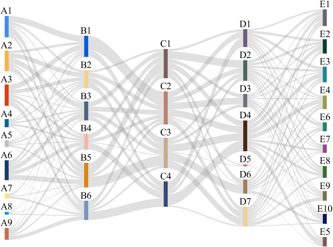
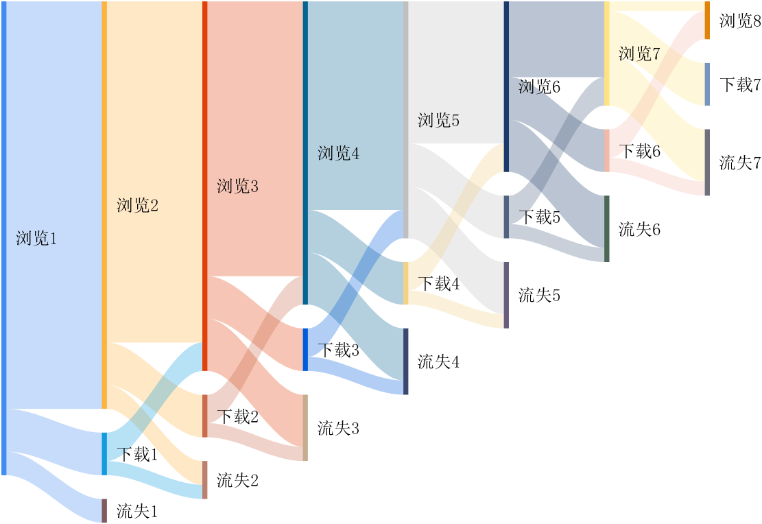
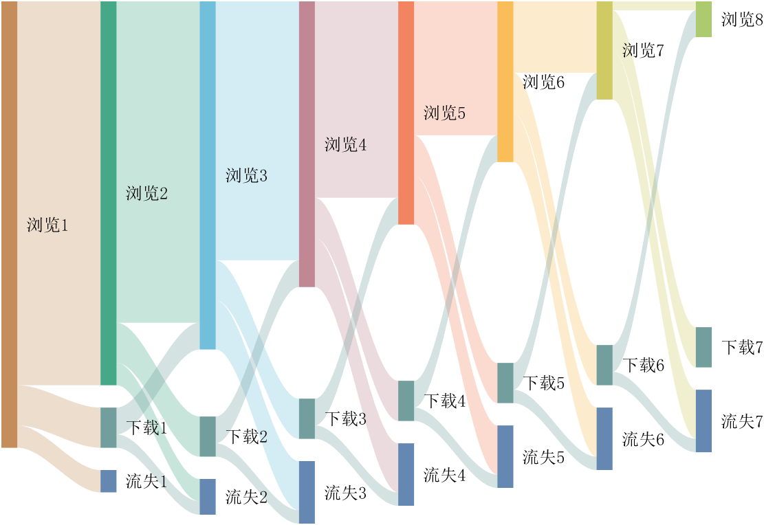
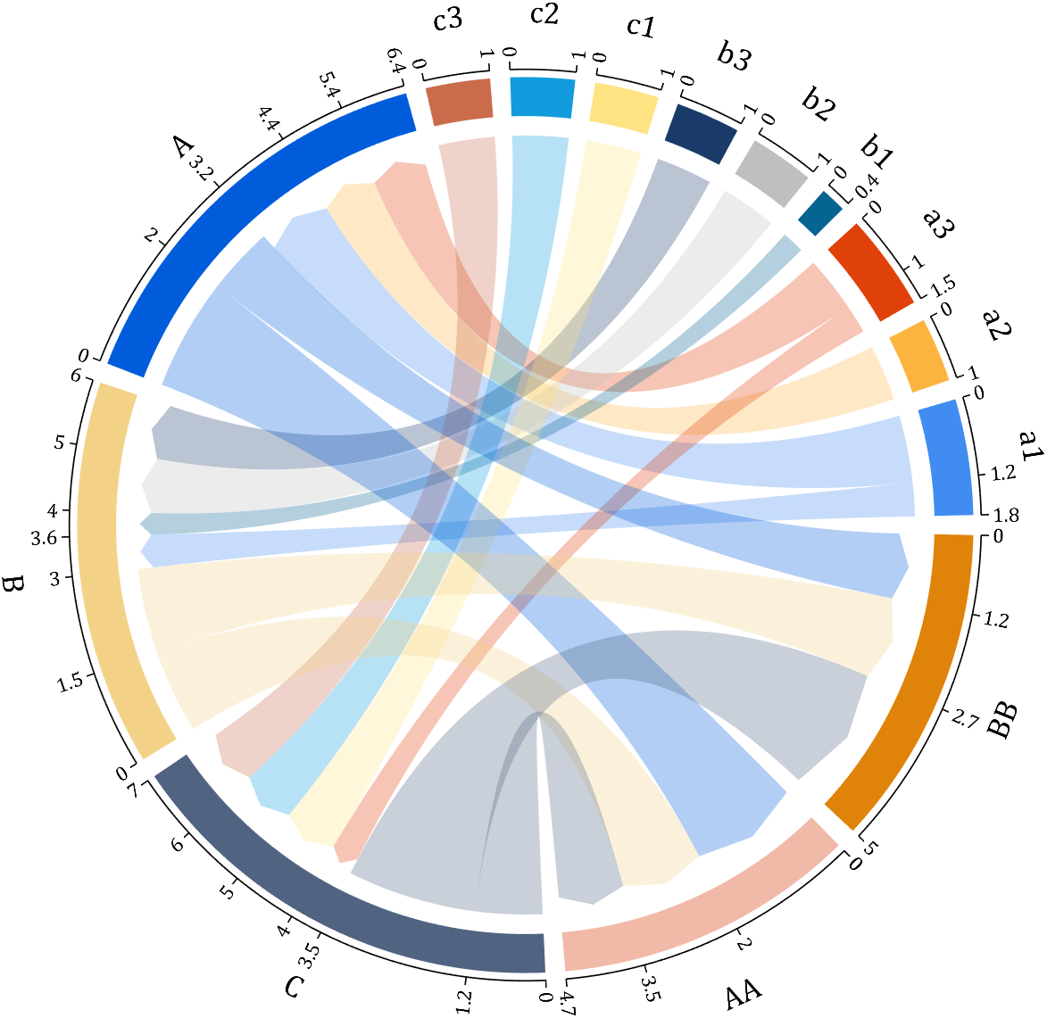
code is here
You can also see the animated version of the competition here
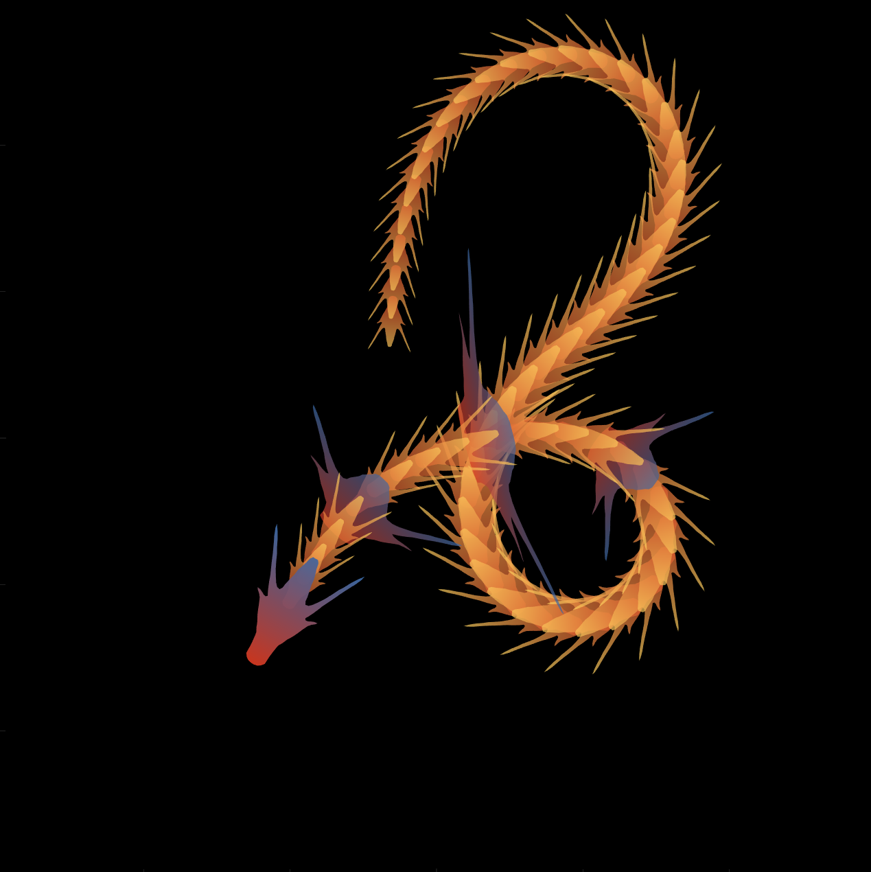

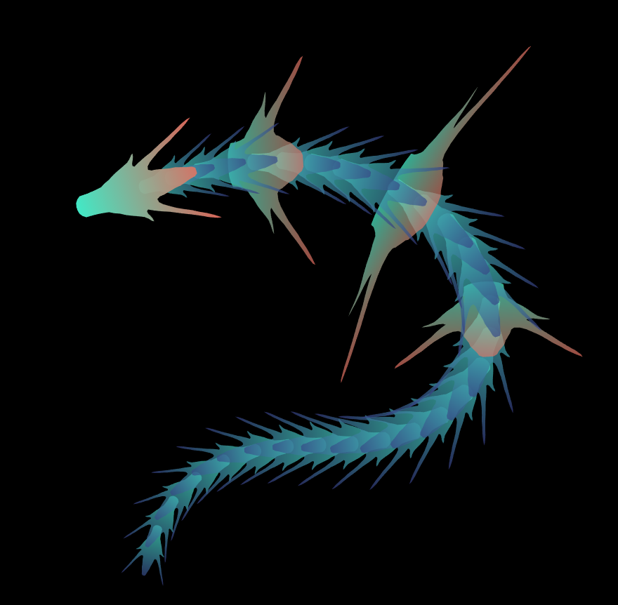
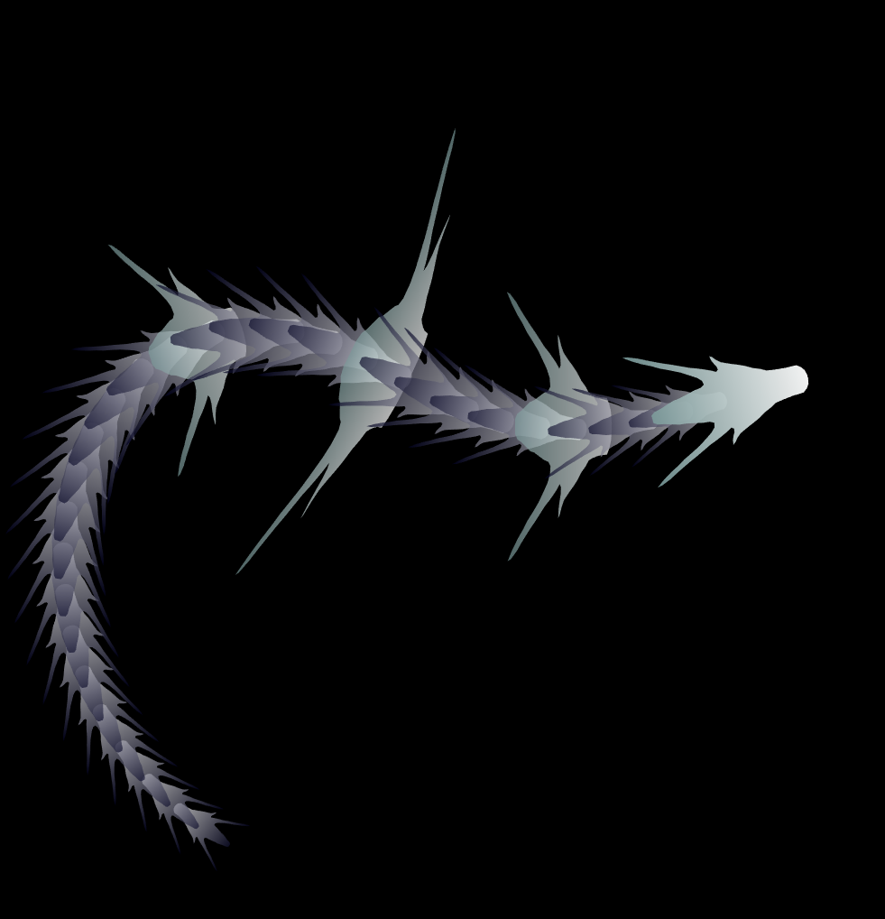
function dragon24
% Copyright (c) 2024, Zhaoxu Liu / slandarer
baseV=[ -.016,.822; -.074,.809; -.114,.781; -.147,.738; -.149,.687; -.150,.630;
-.157,.554; -.166,.482; -.176,.425; -.208,.368; -.237,.298; -.284,.216;
-.317,.143; -.338,.091; -.362,.037;-.382,-.006;-.420,-.051;-.460,-.084;
-.477,-.110;-.430,-.103;-.387,-.084;-.352,-.065;-.317,-.060;-.300,-.082;
-.331,-.139;-.359,-.201;-.385,-.262;-.415,-.342;-.451,-.418;-.494,-.510;
-.533,-.599;-.569,-.675;-.607,-.753;-.647,-.829;-.689,-.932;-.699,-.988;
-.639,-.905;-.581,-.809;-.534,-.717;-.489,-.642;-.442,-.543;-.393,-.447;
-.339,-.362;-.295,-.296;-.251,-.251;-.206,-.241;-.183,-.281;-.175,-.350;
-.156,-.434;-.136,-.521;-.128,-.594;-.103,-.677;-.083,-.739;-.067,-.813;-.039,-.852];
% 基础比例、上色方式数据
baseV=[0,.82;baseV;baseV(end:-1:1,:).*[-1,1];0,.82];
baseV=baseV-mean(baseV,1);
baseF=1:size(baseV,1);
baseY=baseV(:,2);
baseY=(baseY-min(baseY))./(max(baseY)-min(baseY));
N=30;
baseR=sin(linspace(pi/4,5*pi/6,N))./1.2;
baseR=[baseR',baseR'];baseR(1,:)=[1,1];
baseR(5,:)=[2,.6];
baseR(10,:)=[3.7,.4];
baseR(15,:)=[1.8,.6];
baseT=[zeros(N,1),ones(N,1)];
baseM=zeros(N,2);
baseD=baseM;
ratioT=@(Mat,t)Mat*[cos(t),sin(t);-sin(t),cos(t)];
% 配色数据
CList=[211,56,32;56,105,166;253,209,95]./255;
% CList=bone(4);CList=CList(2:4,:);
% CList=flipud(bone(3));
% CList=lines(3);
% CList=colorcube(3);
% CList=rand(3)
baseC1=CList(2,:)+baseY.*(CList(1,:)-CList(2,:));
baseC2=CList(3,:)+baseY.*(CList(1,:)-CList(3,:));
% 构建图窗
fig=figure('units','normalized','position',[.1,.1,.5,.8],...
'UserData',[98,121,32,115,108,97,110,100,97,114,101,114]);
axes('parent',fig,'NextPlot','add','Color',[0,0,0],...
'DataAspectRatio',[1,1,1],'XLim',[-6,6],'YLim',[-6,6],'Position',[0,0,1,1]);
% 构造龙每个部分句柄
dragonHdl(1)=patch('Faces',baseF,'Vertices',baseV,'FaceVertexCData',baseC1,'FaceColor','interp','EdgeColor','none','FaceAlpha',.95);disp(char(fig.UserData))
for i=2:N
dragonHdl(i)=patch('Faces',baseF,'Vertices',baseV.*baseR(i,:)-[0,i./2.5-.3],'FaceVertexCData',baseC2,'FaceColor','interp','EdgeColor','none','FaceAlpha',.7);
end
set(dragonHdl(5),'FaceVertexCData',baseC1,'FaceAlpha',.7)
set(dragonHdl(10),'FaceVertexCData',baseC1,'FaceAlpha',.7)
set(dragonHdl(15),'FaceVertexCData',baseC1,'FaceAlpha',.7)
for i=N:-1:1,uistack(dragonHdl(i),'top');end
for i=1:N
baseM(i,:)=mean(get(dragonHdl(i),'Vertices'),1);
end
baseD=diff(baseM(:,2));Pos=[0,2];
% 主循环及旋转、运动计算
set(gcf,'WindowButtonMotionFcn',@dragonFcn)
fps=8;
game=timer('ExecutionMode', 'FixedRate', 'Period',1/fps, 'TimerFcn', @dragonGame);
start(game)
% Copyright (c) 2023, Zhaoxu Liu / slandarer
set(gcf,'tag','co','CloseRequestFcn',@clo);
function clo(~,~)
stop(game);delete(findobj('tag','co'));clf;close
end
function dragonGame(~,~)
Dir=Pos-baseM(1,:);
Dir=Dir./norm(Dir);
baseT=(baseT(1:end,:)+[Dir;baseT(1:end-1,:)])./2;
baseT=baseT./(vecnorm(baseT')');
theta=atan2(baseT(:,2),baseT(:,1))-pi/2;
baseM(1,:)=baseM(1,:)+(Pos-baseM(1,:))./30;
baseM(2:end,:)=baseM(1,:)+[cumsum(baseD.*baseT(2:end,1)),cumsum(baseD.*baseT(2:end,2))];
for ii=1:N
set(dragonHdl(ii),'Vertices',ratioT(baseV.*baseR(ii,:),theta(ii))+baseM(ii,:))
end
end
function dragonFcn(~,~)
xy=get(gca,'CurrentPoint');
x=xy(1,1);y=xy(1,2);
Pos=[x,y];
Pos(Pos>6)=6;
Pos(Pos<-6)=6;
end
end
There will be a warning when we try to solve equations with piecewise:
syms x y
a = x+y;
b = 1.*(x > 0) + 2.*(x <= 0);
eqns = [a + b*x == 1, a - b == 2];
S = solve(eqns, [x y]);
% 错误使用 mupadengine/feval_internal
% System contains an equation of an unknown type.
%
% 出错 sym/solve (第 293 行)
% sol = eng.feval_internal('solve', eqns, vars, solveOptions);
%
% 出错 demo3 (第 5 行)
% S=solve(eqns,[x y]);
But I found that the solve function can include functions such as heaviside to indicate positive and negative:
syms x y
a = x+y;
b = floor(heaviside(x)) - 2*abs(2*heaviside(x) - 1) + 2*floor(-heaviside(x)) + 4;
eqns = [a + b*x == 1, a - b == 2];
S = solve(eqns, [x y])
% S =
% 包含以下字段的 struct:
%
% x: -3/2
% y: 11/2
The piecewise function is divided into two sections, which is so complex, so this work must be encapsulated as a function to complete:
function pwFunc=piecewiseSym(x,waypoint,func,pfunc)
% @author : slandarer
gSign=[1,heaviside(x-waypoint)*2-1];
lSign=[heaviside(waypoint-x)*2-1,1];
inSign=floor((gSign+lSign)/2);
onSign=1-abs(gSign(2:end));
inFunc=inSign.*func;
onFunc=onSign.*pfunc;
pwFunc=simplify(sum(inFunc)+sum(onFunc));
end
Function Introduction
- x : Argument
- waypoint : Segmentation point of piecewise function
- func : Functions on each segment
- pfunc : The value at the segmentation point
example
syms x
% x waypoint func pfunc
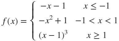
f=piecewiseSym(x,[-1,1],[-x-1,-x^2+1,(x-1)^3],[-x-1,(x-1)^3]);
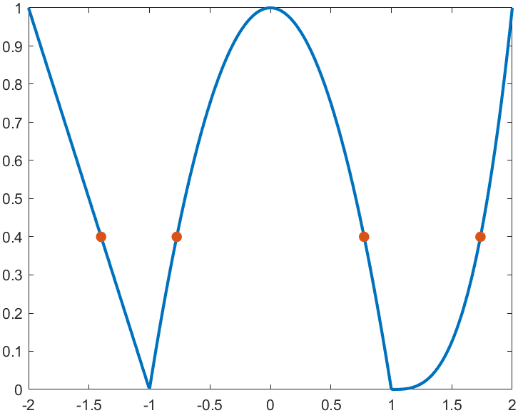
For example, find the analytical solution of the intersection point between the piecewise function and f=0.4 and plot it:
syms x
% x waypoint func pfunc
f=piecewiseSym(x,[-1,1],[-x-1,-x^2+1,(x-1)^3],[-x-1,(x-1)^3]);
% solve
S=solve(f==.4,x)
% S =
%
% -7/5
% (2^(1/3)*5^(2/3))/5 + 1
% -15^(1/2)/5
% 15^(1/2)/5
% draw
xx=linspace(-2,2,500);
f=matlabFunction(f);
yy=f(xx);
plot(xx,yy,'LineWidth',2);
hold on
scatter(double(S),.4.*ones(length(S),1),50,'filled')
precedent
syms x y
a=x+y;
b=piecewiseSym(x,0,[2,1],2);
eqns = [a + b*x == 1, a - b == 2];
S=solve(eqns,[x y])
% S =
% 包含以下字段的 struct:
%
% x: -3/2
% y: 11/2
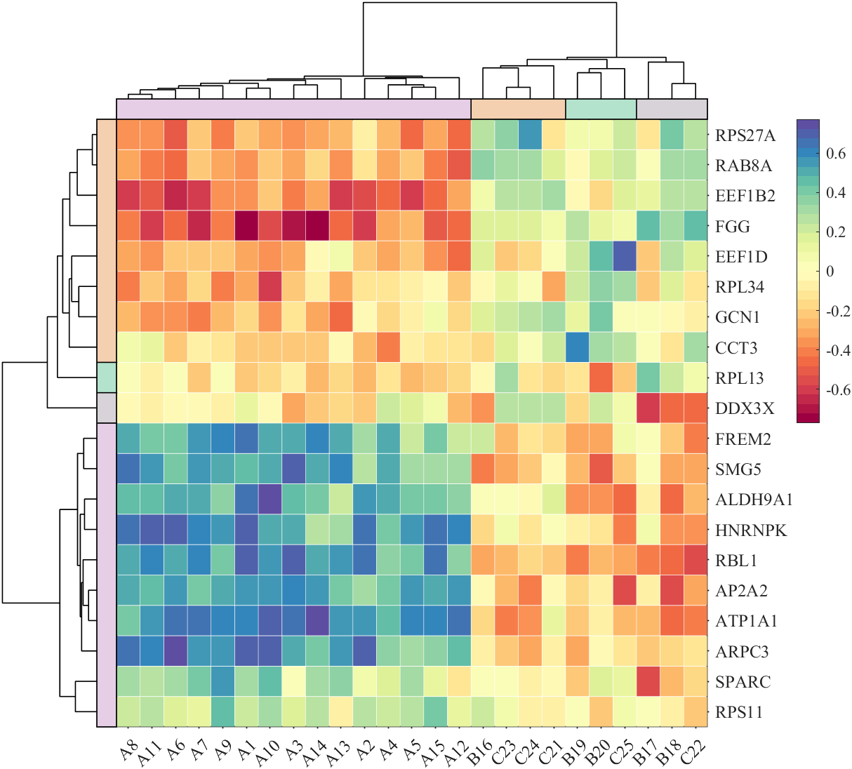
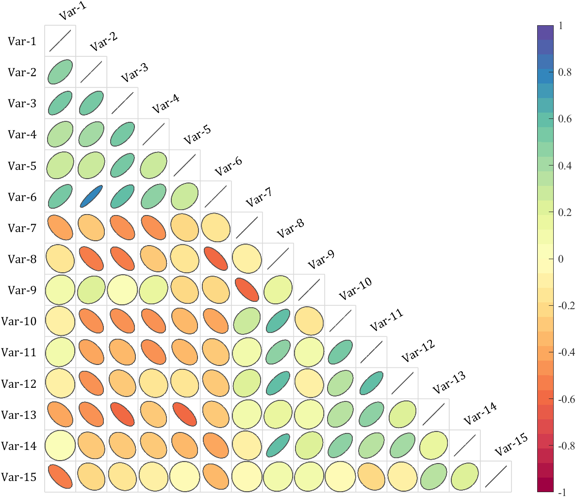
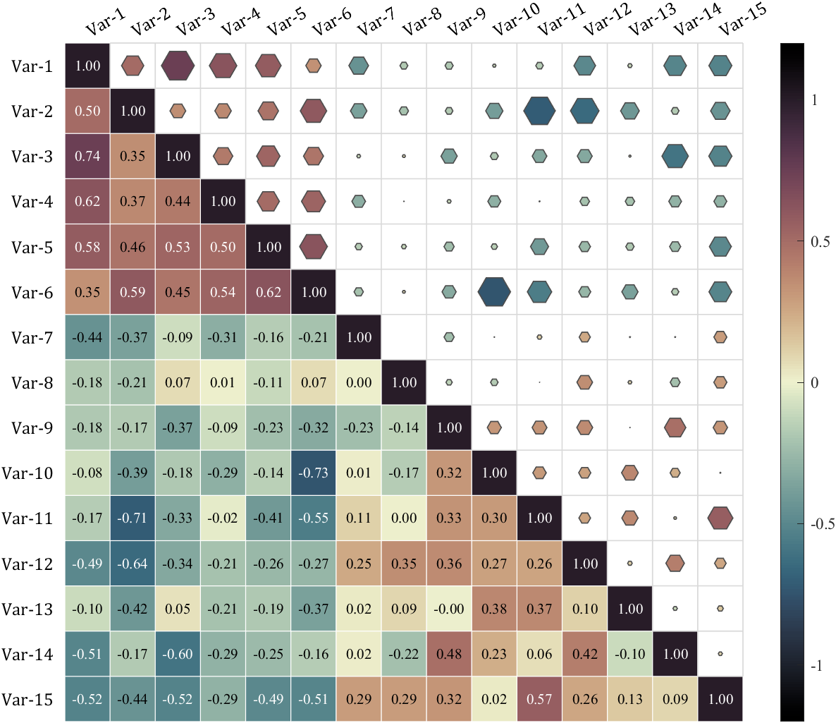
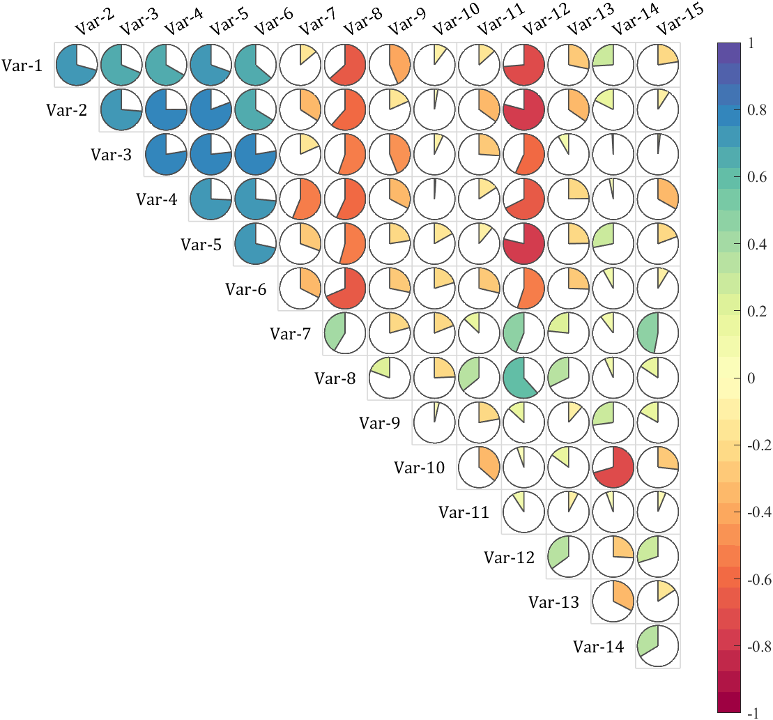
It is pretty easy to draw a cool heatmap for I have uploaded a tool to fileexchange:
您也可以从以下列表中选择网站:
美洲
- América Latina (Español)
- Canada (English)
- United States (English)
欧洲
- Belgium (English)
- Denmark (English)
- Deutschland (Deutsch)
- España (Español)
- Finland (English)
- France (Français)
- Ireland (English)
- Italia (Italiano)
- Luxembourg (English)
- Netherlands (English)
- Norway (English)
- Österreich (Deutsch)
- Portugal (English)
- Sweden (English)
- Switzerland
- United Kingdom(English)
亚太
- Australia (English)
- India (English)
- New Zealand (English)
- 中国
- 日本Japanese (日本語)
- 한국Korean (한국어)