eqn =
搜索
MATLAB FEX(MATLAB File Exchange) should support Markdown syntax for writing. In recent years, many open-source community documentation platforms, such as GitHub, have generally supported Markdown. MATLAB is also gradually improving its support for Markdown syntax. However, when directly uploading files to the MATLAB FEX community and preparing to write an overview, the outdated document format buttons are still present. Even when directly uploading a Markdown document, it cannot be rendered. We hope the community can support Markdown syntax!
BTW,I know that open-source Markdown writing on GitHub and linking to MATLAB FEX is feasible, but this is a workaround. It would be even better if direct native support were available.
Too small
22%
Just right
38%
Too large
40%
2648 个投票
In one of my MATLAB projects, I want to add a button to an existing axes toolbar. The function for doing this is axtoolbarbtn:
axtoolbarbtn(tb,style,Name=Value)
However, I have found that the existing interfaces and behavior make it quite awkward to accomplish this task.
Here are my observations.
Adding a Button to the Default Axes Toolbar Is Unsupported
plot(1:10)
ax = gca;
tb = ax.Toolbar
Calling axtoolbarbtn on ax results in an error:
>> axtoolbarbtn(tb,"state")
Error using axtoolbarbtn (line 77)
Modifying the default axes toolbar is not supported.
Default Axes Toolbar Can't Be Distinguished from an Empty Toolbar
The Children property of the default axes toolbar is empty. Thus, it appears programmatically to have no buttons, just like an empty toolbar created by axtoolbar.
cla
plot(1:10)
ax = gca;
tb = ax.Toolbar;
tb.Children
ans = 0x0 empty GraphicsPlaceholder array.
tb2 = axtoolbar(ax);
tb2.Children
ans = 0x0 empty GraphicsPlaceholder array.
A Workaround
An empty axes toolbar seems to have no use except to initalize a toolbar before immediately adding buttons to it. Therefore, it seems reasonable to assume that an axes toolbar that appears to be empty is really the default toolbar. While we can't add buttons to the default axes toolbar, we can create a new toolbar that has all the same buttons as the default one, using axtoolbar("default"). And then we can add buttons to the new toolbar.
That observation leads to this workaround:
tb = ax.Toolbar;
if isempty(tb.Children)
% Assume tb is the default axes toolbar. Recreate
% it with the default buttons so that we can add a new
% button.
tb = axtoolbar(ax,"default");
end
btn = axtoolbarbtn(tb);
% Then set up the button as desired (icon, callback,
% etc.) by setting its properties.
As workarounds go, it's not horrible. It just seems a shame to have to delete and then recreate a toolbar just to be able to add a button to it.
The worst part about the workaround is that it is so not obvious. It took me a long time of experimentation to figure it out, including briefly giving it up as seemingly impossible.
The documentation for axtoolbarbtn avoids the issue. The most obvious example to write for axtoolbarbtn would be the first thing every user of it will try: add a toolbar button to the toolbar that gets created automatically in every call to plot. The doc page doesn't include that example, of course, because it wouldn't work.
My Request
I like the axes toolbar concept and the axes interactivity that it promotes, and I think the programming interface design is mostly effective. My request to MathWorks is to modify this interface to smooth out the behavior discontinuity of the default axes toolbar, with an eye towards satisfying (and documenting) the general use case that I've described here.
One possible function design solution is to make the default axes toolbar look and behave like the toolbar created by axtoolbar("default"), so that it has Children and so it is modifiable.
I am curious as to how my goal can be accomplished in Matlab.
The present APP called "Matching Network Designer" works quite well, but it is limited to a single section of a "PI", a "TEE", or an "L" topology circuit.
This limits the bandwidth capability of the APP when the intended use is to create an amplifier design intended for wider bandwidth projects.
I am requesting that a "Broadband Matching Network Designer" APP be developed by you, the MathWorks support team.
One suggestion from me is to be able to cascade a second section (or "pole") to the first.
Then the resulting topology would be capable of achieving that wider bandwidth of the microwave amplifier project where it would be later used with the transistor output and input matching networks.
Instead of limiting the APP to a single frequency, the entire s parameter file would be used as an input.
The APP would convert the polar s parameters to rectangular scaler complex impedances that you already use.
At that point, having started out with the first initial center frequency, the other frequencies both greater than and less than the center would come into use by an optimization of the circuit elements.
I'm hoping that you will be able to take on this project.
I can include an attachment of such a Matching Network Designer APP that you presently have if you like.
That network is centered at 10 GHz.
Kimberly Renee Alvarez.
310-367-5768
Hello,
Now that the "Copilot+PC" (Windows ARM) laptops are rapidly increasing in market share (Microsoft Surface Laptop, Dell XPS 13, HP OmniBook X 14, and more), are there any plans to provide builds for Matlab on Windows arm64?
Since there are already Windows builds of Matlab, it shouldn't be too hard to compile for Windows arm64, as far as I know. But I am not famaliar with Matlab's codebase.
Please try to publish Windows arm64 builds soon so that Matlab can be much more usable on Windows on ARM as it will run natively instead of in emulation.
Thank you very much.
If you have a folder with an enormous number of files and want to use the uigetfile function to select specific files, you may have noticed a significant delay in displaying the file list.
Thanks to the assistance from MathWorks support, an interesting behavior was observed.
For example, if a folder such as Z:\Folder1\Folder2\data contains approximately 2 million files, and you attempt to use uigetfile to access files with a specific extension (e.g., *.ext), the following behavior occurs:
Method 1: This takes minutes to show me the list of all files
[FileName, PathName] = uigetfile('Z:\Folder1\Folder2\data\*.ext', 'File selection');
Method 2: This takes less than a second to display all files.
[FileName, PathName] = uigetfile('*.ext', 'File selection','Z:\Folder1\Folder2\data');
Method 3: This method also takes minutes to display the file list. What is intertesting is that this method is the same as Method 2, except that a file seperator "\" is added at the end of the folder string.
[FileName, PathName] = uigetfile('*.ext', 'File selection','Z:\Folder1\Folder2\data\');
I was informed that the Mathworks development team has been informed of this strange behaviour.
I am using 2023a, but think this should be the same for newer versions.
This post is more of a "tips and tricks" guide than a question.
If you have a folder with an enormous number of files and want to use the uigetfile function to select specific files, you may have noticed a significant delay in displaying the file list.
Thanks to the assistance from MathWorks support, an interesting behavior was observed.
For example, if a folder such as Z:\Folder1\Folder2\data contains approximately 2 million files, and you attempt to use uigetfile to access files with a specific extension (e.g., *.ext), the following behavior occurs:
Method 1: This takes minutes to show me the list of all files
[FileName, PathName] = uigetfile('Z:\Folder1\Folder2\data\*.ext', 'File selection');
Method 2: This takes less than a second to display all files.
[FileName, PathName] = uigetfile('*.ext', 'File selection','Z:\Folder1\Folder2\data');
Method 3: This method also takes minutes to display the file list. What is intertesting is that this method is the same as Method 2, except that a file seperator "\" is added at the end of the folder string.
[FileName, PathName] = uigetfile('*.ext', 'File selection','Z:\Folder1\Folder2\data\');
I was informed that the Mathworks development team has been informed of this strange behaviour.
I am using 2023a, but think this should be the same for newer versions.

Christmas is coming, here are two dynamic Christmas tree drawing codes:
Crystal XMas Tree
function XmasTree2024_1
fig = figure('Units','normalized', 'Position',[.1,.1,.5,.8],...
'Color',[0,9,33]/255, 'UserData',40 + [60,65,75,72,0,59,64,57,74,0,63,59,57,0,1,6,45,75,61,74,28,57,76,57,1,1]);
axes('Parent',fig, 'Position',[0,-1/6,1,1+1/3], 'UserData',97 + [18,11,0,13,3,0,17,4,17],...
'XLim',[-1.5,1.5], 'YLim',[-1.5,1.5], 'ZLim',[-.2,3.8], 'DataAspectRatio', [1,1,1], 'NextPlot','add',...
'Projection','perspective', 'Color',[0,9,33]/255, 'XColor','none', 'YColor','none', 'ZColor','none')
%% Draw Christmas tree
F = [1,3,4;1,4,5;1,5,6;1,6,3;...
2,3,4;2,4,5;2,5,6;2,6,3];
dP = @(V) patch('Faces',F, 'Vertices',V, 'FaceColor',[0 71 177]./255,...
'FaceAlpha',rand(1).*0.2+0.1, 'EdgeColor',[0 71 177]./255.*0.8,...
'EdgeAlpha',0.6, 'LineWidth',0.5, 'EdgeLighting','gouraud', 'SpecularStrength',0.3);
r = .1; h = .8;
V0 = [0,0,0; 0,0,1; 0,r,h; r,0,h; 0,-r,h; -r,0,h];
% Rotation matrix
Rx = @(V, theta) V*[1 0 0; 0 cos(theta) sin(theta); 0 -sin(theta) cos(theta)];
Rz = @(V, theta) V*[cos(theta) sin(theta) 0;-sin(theta) cos(theta) 0; 0 0 1];
N = 180; Vn = zeros(N, 3); eval(char(fig.UserData))
for i = 1:N
tV = Rz(Rx(V0.*(1.2 - .8.*i./N + rand(1).*.1./i^(1/5)), pi/3.*(1 - .6.*i./N)), i.*pi/8.1 + .001.*i.^2) + [0,0,.016.*i];
dP(tV); Vn(i,:) = tV(2,:);
end
scatter3(Vn(:,1).*1.02,Vn(:,2).*1.02,Vn(:,3).*1.01, 30, 'w', 'Marker','*', 'MarkerEdgeAlpha',.5)
%% Draw Star of Bethlehem
w = .3; R = .62; r = .4; T = (1/8:1/8:(2 - 1/8)).'.*pi;
V8 = [ 0, 0, w; 0, 0,-w;
1, 0, 0; 0, 1, 0; -1, 0, 0; 0,-1,0;
R, R, 0; -R, R, 0; -R,-R, 0; R,-R,0;
cos(T).*r, sin(T).*r, T.*0];
F8 = [1,3,25; 1,3,11; 2,3,25; 2,3,11; 1,7,11; 1,7,13; 2,7,11; 2,7,13;
1,4,13; 1,4,15; 2,4,13; 2,4,15; 1,8,15; 1,8,17; 2,8,15; 2,8,17;
1,5,17; 1,5,19; 2,5,17; 2,5,19; 1,9,19; 1,9,21; 2,9,19; 2,9,21;
1,6,21; 1,6,23; 2,6,21; 2,6,23; 1,10,23; 1,10,25; 2,10,23; 2,10,25];
V8 = Rx(V8.*.3, pi/2) + [0,0,3.5];
patch('Faces',F8, 'Vertices',V8, 'FaceColor',[255,223,153]./255,...
'EdgeColor',[255,223,153]./255, 'FaceAlpha', .2)
%% Draw snow
sXYZ = rand(200,3).*[4,4,5] - [2,2,0];
sHdl1 = plot3(sXYZ(1:90,1),sXYZ(1:90,2),sXYZ(1:90,3), '*', 'Color',[.8,.8,.8]);
sHdl2 = plot3(sXYZ(91:200,1),sXYZ(91:200,2),sXYZ(91:200,3), '.', 'Color',[.6,.6,.6]);
annotation(fig,'textbox',[0,.05,1,.09], 'Color',[1 1 1], 'String','Merry Christmas Matlaber',...
'HorizontalAlignment','center', 'FontWeight','bold', 'FontSize',48,...
'FontName','Times New Roman', 'FontAngle','italic', 'FitBoxToText','off','EdgeColor','none');
% Rotate the Christmas tree and let the snow fall
for i=1:1e8
sXYZ(:,3) = sXYZ(:,3) - [.05.*ones(90,1); .06.*ones(110,1)];
sXYZ(sXYZ(:,3)<0, 3) = sXYZ(sXYZ(:,3) < 0, 3) + 5;
sHdl1.ZData = sXYZ(1:90,3); sHdl2.ZData = sXYZ(91:200,3);
view([i,30]); drawnow; pause(.05)
end
end

Curved XMas Tree
function XmasTree2024_2
fig = figure('Units','normalized', 'Position',[.1,.1,.5,.8],...
'Color',[0,9,33]/255, 'UserData',40 + [60,65,75,72,0,59,64,57,74,0,63,59,57,0,1,6,45,75,61,74,28,57,76,57,1,1]);
axes('Parent',fig, 'Position',[0,-1/6,1,1+1/3], 'UserData',97 + [18,11,0,13,3,0,17,4,17],...
'XLim',[-6,6], 'YLim',[-6,6], 'ZLim',[-16, 1], 'DataAspectRatio', [1,1,1], 'NextPlot','add',...
'Projection','perspective', 'Color',[0,9,33]/255, 'XColor','none', 'YColor','none', 'ZColor','none')
%% Draw Christmas tree
[X,T] = meshgrid(.4:.1:1, 0:pi/50:2*pi);
XM = 1 + sin(8.*T).*.05;
X = X.*XM; R = X.^(3).*(.5 + sin(8.*T).*.02);
dF = @(R, T, X) surf(R.*cos(T), R.*sin(T), -X, 'EdgeColor',[20,107,58]./255,...
'FaceColor', [20,107,58]./255, 'FaceAlpha',.2, 'LineWidth',1);
CList = [254,103,110; 255,191,115; 57,120,164]./255;
for i = 1:5
tR = R.*(2 + i); tT = T+i; tX = X.*(2 + i) + i;
SFHdl = dF(tR, tT, tX);
[~, ind] = sort(SFHdl.ZData(:)); ind = ind(1:8);
C = CList(randi([1,size(CList,1)], [8,1]), :);
scatter3(tR(ind).*cos(tT(ind)), tR(ind).*sin(tT(ind)), -tX(ind), 120, 'filled',...
'CData', C, 'MarkerEdgeColor','none', 'MarkerFaceAlpha',.3)
scatter3(tR(ind).*cos(tT(ind)), tR(ind).*sin(tT(ind)), -tX(ind), 60, 'filled', 'CData', C)
end
%% Draw Star of Bethlehem
Rx = @(V, theta) V*[1 0 0; 0 cos(theta) sin(theta); 0 -sin(theta) cos(theta)];
% Rz = @(V, theta) V*[cos(theta) sin(theta) 0;-sin(theta) cos(theta) 0; 0 0 1];
w = .3; R = .62; r = .4; T = (1/8:1/8:(2 - 1/8)).'.*pi;
V8 = [ 0, 0, w; 0, 0,-w;
1, 0, 0; 0, 1, 0; -1, 0, 0; 0,-1,0;
R, R, 0; -R, R, 0; -R,-R, 0; R,-R,0;
cos(T).*r, sin(T).*r, T.*0];
F8 = [1,3,25; 1,3,11; 2,3,25; 2,3,11; 1,7,11; 1,7,13; 2,7,11; 2,7,13;
1,4,13; 1,4,15; 2,4,13; 2,4,15; 1,8,15; 1,8,17; 2,8,15; 2,8,17;
1,5,17; 1,5,19; 2,5,17; 2,5,19; 1,9,19; 1,9,21; 2,9,19; 2,9,21;
1,6,21; 1,6,23; 2,6,21; 2,6,23; 1,10,23; 1,10,25; 2,10,23; 2,10,25];
V8 = Rx(V8.*.8, pi/2) + [0,0,-1.3];
patch('Faces',F8, 'Vertices',V8, 'FaceColor',[255,223,153]./255,...
'EdgeColor',[255,223,153]./255, 'FaceAlpha', .2)
annotation(fig,'textbox',[0,.05,1,.09], 'Color',[1 1 1], 'String','Merry Christmas Matlaber',...
'HorizontalAlignment','center', 'FontWeight','bold', 'FontSize',48,...
'FontName','Times New Roman', 'FontAngle','italic', 'FitBoxToText','off','EdgeColor','none');
%% Draw snow
sXYZ = rand(200,3).*[12,12,17] - [6,6,16];
sHdl1 = plot3(sXYZ(1:90,1),sXYZ(1:90,2),sXYZ(1:90,3), '*', 'Color',[.8,.8,.8]);
sHdl2 = plot3(sXYZ(91:200,1),sXYZ(91:200,2),sXYZ(91:200,3), '.', 'Color',[.6,.6,.6]);
for i=1:1e8
sXYZ(:,3) = sXYZ(:,3) - [.1.*ones(90,1); .12.*ones(110,1)];
sXYZ(sXYZ(:,3)<-16, 3) = sXYZ(sXYZ(:,3) < -16, 3) + 17.5;
sHdl1.ZData = sXYZ(1:90,3); sHdl2.ZData = sXYZ(91:200,3);
view([i,30]); drawnow; pause(.05)
end
end
I wish all MATLABers a Merry Christmas in advance!
Speaking as someone with 31+ years of experience developing and using imshow, I want to advocate for retiring and replacing it.
The function imshow has behaviors and defaults that were appropriate for the MATLAB and computer monitors of the 1990s, but which are not the best choice for most image display situations in today's MATLAB. Also, the 31 years have not been kind to the imshow code base. It is a glitchy, hard-to-maintain monster.
My new File Exchange function, imview, illustrates the kind of changes that I think should be made. The function imview is a much better MATLAB graphics citizen and produces higher quality image display by default, and it dispenses with the whole fraught business of trying to resize the containing figure. Although this is an initial release that does not yet support all the useful options that imshow does, it does enough that I am prepared to stop using imshow in my own work.
The Image Processing Toolbox team has just introduced in R2024b a new image viewer called imageshow, but that image viewer is created in a special-purpose window. It does not satisfy the need for an image display function that works well with the axes and figure objects of the traditional MATLAB graphics system.
I have published a blog post today that describes all this in more detail. I'd be interested to hear what other people think.
Note: Yes, I know there is an Image Processing Toolbox function called imview. That one is a stub for an old toolbox capability that was removed something like 15+ years ago. The only thing the toolbox imview function does now is call error. I have just submitted a support request to MathWorks to remove this old stub.
The int function in the Symbolic Toolbox has a hold/release functionality wherein the expression can be held to delay evaluation
syms x I
eqn = I == int(x,x,'Hold',true)
which allows one to show the integral, and then use release to show the result
release(eqn)
Maybe it would be nice to be able to hold/release any symbolic expression to delay the engine from doing evaluations/simplifications that it typically does. For example:
x*(x+1)/x, sin(sym(pi)/3)

If I'm trying to show a sequence of steps to develop a result, maybe I want to explicitly keep the x/x in the first case and then say "now the x in the numerator and denominator cancel and the result is ..." followed by the release command to get the final result.
Perhaps held expressions could even be nested to show a sequence of results upon subsequent releases.
Held expressions might be subject to other limitations, like maybe they can't be fplotted.
Seems like such a capability might not be useful for problem solving, but might be useful for exposition, instruction, etc.
Hi! My name is Mike McLernon, and I’m a product marketing engineer with MathWorks. In my role, I look at the trends ongoing in the wireless industry, across lots of different standards (think 5G, WLAN, SatCom, Bluetooth, etc.), and I seek to shape and guide the software that MathWorks builds to respond to these trends. That’s all about communicating within the Mathworks organization, but every so often it’s worth communicating these trends to our audience in the world at large. Many of the people reading this are engineers (or engineers at heart), and we all want to know what’s happening in the geek world around us. I think that now is one of these times to communicate an important milestone. So, without further ado . . .
Bluetooth 6.0 is here! Announced in September by the Bluetooth Special Interest Group (SIG), it’s making more advances in its quest to create a “world without wires”. A few of the salient features in Bluetooth 6.0 are:
- Channel sounding (for accurate distance measurements)
- Decision-based advertising filtering (for more efficient channel scanning)
- Monitoring advertisers (for improved energy efficiency when devices come into and go out of range)
- Frame space updates (for both higher throughput and better coexistence management)
Bluetooth 6.0 includes other features as well, but the SIG has put special promotional emphasis on channel sounding (CS), which once upon a time was called High Accuracy Distance Measurement (HADM). The SIG has said that CS is a step towards true distance awareness, and 10 cm ranging accuracy. I think their emphasis is in exactly the right place, so let’s learn more about this technology and how it is used.
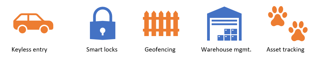
CS can be used for the following use cases:
- Keyless vehicle entry, performed by communication between a key fob or phone and the car’s anchor points
- Smart locks, to permit access only when an authorized device is within a designated proximity to the locks
- Geofencing, to limit access to designated areas
- Warehouse management, to monitor inventory and manage logistics
- Asset tracking for virtually any object of interest
In the past, Bluetooth devices would use a received signal strength indicator (RSSI) measurement to infer the distance between two of them. They would assume a free space path loss on the link, and use a straightforward equation to estimate distance:
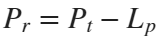
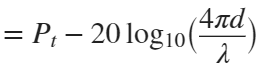
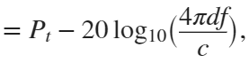 where
whereSo in this method, 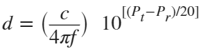 . But if the signal suffers more loss from multipath or shadowing, then the distance would be overestimated. Something better needed to be found.
. But if the signal suffers more loss from multipath or shadowing, then the distance would be overestimated. Something better needed to be found.Bluetooth 6.0 introduces not one, but two ways to accurately measure distance:
- Round-trip time (RTT) measurement
- Phase-based ranging (PBR) measurement
The RTT measurement method uses the fact that the Bluetooth signal time of flight (TOF) between two devices is half the RTT. It can then accurately compute the distance d as
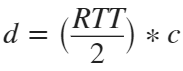 , where c is again the speed of light. This method requires accurate measurements of the time of departure (TOD) of the outbound signal from device 1 (the Initiator), time of arrival (TOA) of the outbound signal to device 2 (the Reflector), TOD of the return signal from device 2, and TOA of the return signal to device 1. The diagram below shows the signal paths and the times.
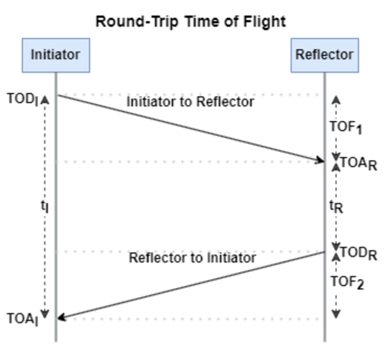
If you want to see how you can use MATLAB to simulate the RTT method, take a look at Estimate Distance Between Bluetooth LE Devices by Using Channel Sounding and Round-Trip Timing.
The PBR method uses two Bluetooth signals of different frequencies to measure distance. These signals are simply tones – sine waves. Without going through the derivation, PBR calculates distance d as
The mod() operation is needed to eliminate ambiguities in the distance calculation and the final division by two is to convert a round trip distance to a one-way distance. Because a given phase difference value can hold true for an infinite number of distance values, the mod() operation chooses the smallest distance that satisfies the equation. Also, these tones can be as close as 1 MHz apart. In that case, the maximum resolvable distance measurement is about 150 m. The plot below shows that ambiguity and repetition in distance measurement.
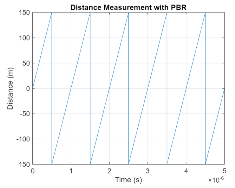
If you want to see how you can use MATLAB to simulate the PBR method, take a look at Estimate Distance Between Bluetooth LE Devices by Using Channel Sounding and Phase-Based Ranging.
Bluetooth 6.0 outlines RTT and PBR distance measurement methods, but CS does not mandate a specific algorithm for calculating distance estimates. This flexibility allows device manufacturers to tailor solutions to various use cases, balancing computational complexity with required accuracy and adapting to different radio environments. Examples include simple phase difference calculations and FFT-based methods.
Although Bluetooth 6.0 is now out, it is far from a finished version. The SIG is actively working through the ratification process for two major extensions:
- High Data Throughput, up to 8 Mbps
- 5 and 6 GHz operation
See the last few minutes of this video from the SIG to learn more about these exciting future developments. And if you want to see more Bluetooth blogs, give a review of this one! Finally, if you have specific Bluetooth questions, give me a shout and let’s start a discussion!
So I made this.
clear
close all
clc
% inspired from: https://www.youtube.com/watch?v=3CuUmy7jX6k
%% user parameters
h = 768;
w = 1024;
N_snowflakes = 50;
%% set figure window
figure(NumberTitle="off", ...
name='Mat-snowfalling-lab (right click to stop)', ...
MenuBar="none")
ax = gca;
ax.XAxisLocation = 'origin';
ax.YAxisLocation = 'origin';
axis equal
axis([0, w, 0, h])
ax.Color = 'k';
ax.XAxis.Visible = 'off';
ax.YAxis.Visible = 'off';
ax.Position = [0, 0, 1, 1];
%% first snowflake
ht = gobjects(1, 1);
for i=1:length(ht)
ht(i) = hgtransform();
ht(i).UserData = snowflake_factory(h, w);
ht(i).Matrix(2, 4) = ht(i).UserData.y;
ht(i).Matrix(1, 4) = ht(i).UserData.x;
im = imagesc(ht(i), ht(i).UserData.img);
im.AlphaData = ht(i).UserData.alpha;
colormap gray
end
%% falling snowflake
tic;
while true
% add a snowflake every 0.3 seconds
if toc > 0.3
if length(ht) < N_snowflakes
ht = [ht; hgtransform()];
ht(end).UserData = snowflake_factory(h, w);
ht(end).Matrix(2, 4) = ht(end).UserData.y;
ht(end).Matrix(1, 4) = ht(end).UserData.x;
im = imagesc(ht(end), ht(end).UserData.img);
im.AlphaData = ht(end).UserData.alpha;
colormap gray
end
tic;
end
ax.CLim = [0, 0.0005]; % prevent from auto clim
% move snowflakes
for i = 1:length(ht)
ht(i).Matrix(2, 4) = ht(i).Matrix(2, 4) + ht(i).UserData.velocity;
end
if strcmp(get(gcf, 'SelectionType'), 'alt')
set(gcf, 'SelectionType', 'normal')
break
end
drawnow
% delete the snowflakes outside the window
for i = length(ht):-1:1
if ht(i).Matrix(2, 4) < -length(ht(i).Children.CData)
delete(ht(i))
ht(i) = [];
end
end
end
%% snowflake factory
function snowflake = snowflake_factory(h, w)
radius = round(rand*h/3 + 10);
sigma = radius/6;
snowflake.velocity = -rand*0.5 - 0.1;
snowflake.x = rand*w;
snowflake.y = h - radius/3;
snowflake.img = fspecial('gaussian', [radius, radius], sigma);
snowflake.alpha = snowflake.img/max(max(snowflake.img));
end
It would be nice to have a function to shade between two curves. This is a common question asked on Answers and there are some File Exchange entries on it but it's such a common thing to want to do I think there should be a built in function for it. I'm thinking of something like
plotsWithShading(x1, y1, 'r-', x2, y2, 'b-', 'ShadingColor', [.7, .5, .3], 'Opacity', 0.5);
So we can specify the coordinates of the two curves, and the shading color to be used, and its opacity, and it would shade the region between the two curves where the x ranges overlap. Other options should also be accepted, like line with, line style, markers or not, etc. Perhaps all those options could be put into a structure as fields, like
plotsWithShading(x1, y1, options1, x2, y2, options2, 'ShadingColor', [.7, .5, .3], 'Opacity', 0.5);
the shading options could also (optionally) be a structure. I know it can be done with a series of other functions like patch or fill, but it's kind of tricky and not obvious as we can see from the number of questions about how to do it.
Does anyone else think this would be a convenient function to add?
In the past two years, large language models have brought us significant changes, leading to the emergence of programming tools such as GitHub Copilot, Tabnine, Kite, CodeGPT, Replit, Cursor, and many others. Most of these tools support code writing by providing auto-completion, prompts, and suggestions, and they can be easily integrated with various IDEs.
As far as I know, aside from the MATLAB-VSCode/MatGPT plugin, MATLAB lacks such AI assistant plugins for its native MATLAB-Desktop, although it can leverage other third-party plugins for intelligent programming assistance. There is hope for a native tool of this kind to be built-in.
Hi everyone, I wrote several fancy functions that may help your coding experience, since they are in very early developing stage, I will be thankful if anyone could try them and give some feedbacks. Currently I have following:
- fstr: a Python f-string like expression
- printf: an easy to use fprintf function, accepts multiple arguments with seperator, end string control.
I will bring more functions or packages like logger when I am available.
The code is open sourced at GitHub with simple examples: https://github.com/bentrainer/MMGA
MATLAB Comprehensive commands list:
- clc - clears command window, workspace not affected
- clear - clears all variables from workspace, all variable values are lost
- diary - records into a file almost everything that appears in command window.
- exit - exits the MATLAB session
- who - prints all variables in the workspace
- whos - prints all variables in current workspace, with additional information.
Ch. 2 - Basics:
- Mathematical constants: pi, i, j, Inf, Nan, realmin, realmax
- Precedence rules: (), ^, negation, */, +-, left-to-right
- and, or, not, xor
- exp - exponential
- log - natural logarithm
- log10 - common logarithm (base 10)
- sqrt (square root)
- fprintf("final amount is %f units.", amt);
- can have: %f, %d, %i, %c, %s
- %f - fixed-point notation
- %e - scientific notation with lowercase e
- disp - outputs to a command window
- % - fieldWith.precision convChar
- MyArray = [startValue : IncrementingValue : terminatingValue]
Linspace
linspace(xStart, xStop, numPoints)
% xStart: Starting value
% xStop: Stop value
% numPoints: Number of linear-spaced points, including xStart and xStop
% Outputs a row array with the resulting values
Logspace
logspace(powerStart, powerStop, numPoints)
% powerStart: Starting value 10^powerStart
% powerStop: Stop value 10^powerStop
% numPoints: Number of logarithmic spaced points, including 10^powerStart and 10^powerStop
% Outputs a row array with the resulting values
- Transpose an array with []'
Element-Wise Operations
rowVecA = [1, 4, 5, 2];
rowVecB = [1, 3, 0, 4];
sumEx = rowVecA + rowVecB % Element-wise addition
diffEx = rowVecA - rowVecB % Element-wise subtraction
dotMul = rowVecA .* rowVecB % Element-wise multiplication
dotDiv = rowVecA ./ rowVecB % Element-wise division
dotPow = rowVecA .^ rowVecB % Element-wise exponentiation
- isinf(A) - check if the array elements are infinity
- isnan(A)
Rounding Functions
- ceil(x) - rounds each element of x to nearest integer >= to element
- floor(x) - rounds each element of x to nearest integer <= to element
- fix(x) - rounds each element of x to nearest integer towards 0
- round(x) - rounds each element of x to nearest integer. if round(x, N), rounds N digits to the right of the decimal point.
- rem(dividend, divisor) - produces a result that is either 0 or has the same sign as the dividen.
- mod(dividend, divisor) - produces a result that is either 0 or same result as divisor.
- Ex: 12/2, 12 is dividend, 2 is divisor
- sum(inputArray) - sums all entires in array
Complex Number Functions
- abs(z) - absolute value, is magnitude of complex number (phasor form r*exp(j0)
- angle(z) - phase angle, corresponds to 0 in r*exp(j0)
- complex(a,b) - creates complex number z = a + jb
- conj(z) - given complex conjugate a - jb
- real(z) - extracts real part from z
- imag(z) - extracts imaginary part from z
- unwrap(z) - removes the modulus 2pi from an array of phase angles.
Statistics Functions
- mean(xAr) - arithmetic mean calculated.
- std(xAr) - calculated standard deviation
- median(xAr) - calculated the median of a list of numbers
- mode(xAr) - calculates the mode, value that appears most often
- max(xAr)
- min(xAr)
- If using &&, this means that if first false, don't bother evaluating second
Random Number Functions
- rand(numRand, 1) - creates column array
- rand(1, numRand) - creates row array, both with numRand elements, between 0 and 1
- randi(maxRandVal, numRan, 1) - creates a column array, with numRand elements, between 1 and maxRandValue.
- randn(numRand, 1) - creates a column array with normally distributed values.
- Ex: 10 * rand(1, 3) + 6
- "10*rand(1, 3)" produces a row array with 3 random numbers between 0 and 10. Adding 6 to each element results in random values between 6 and 16.
- randi(20, 1, 5)
- Generates 5 (last argument) random integers between 1 (second argument) and 20 (first argument). The arguments 1 and 5 specify a 1 × 5 row array is returned.
Discrete Integer Mathematics
- primes(maxVal) - returns prime numbers less than or equal to maxVal
- isprime(inputNums) - returns a logical array, indicating whether each element is a prime number
- factor(intVal) - returns the prime factors of a number
- gcd(aVals, bVals) - largest integer that divides both a and b without a remainder
- lcm(aVals, bVals) - smallest positive integer that is divisible by both a and b
- factorial(intVals) - returns the factorial
- perms(intVals) - returns all the permutations of the elements int he array intVals in a 2D array pMat.
- randperm(maxVal)
- nchoosek(n, k)
- binopdf(x, n, p)
Concatenation
- cat, vertcat, horzcat
- Flattening an array, becomes vertical: sampleList = sampleArray ( : )
Dimensional Properties of Arrays
- nLargest = length(inArray) - number of elements along largest dimension
- nDim = ndims(inArray)
- nArrElement = numel(inArray) - nuber of array elements
- [nRow, nCol] = size(inArray) - returns the number of rows and columns on array. use (inArray, 1) if only row, (inArray, 2) if only column needed
- aZero = zeros(m, n) - creates an m by n array with all elements 0
- aOnes = ones(m, n) - creates an m by n array with all elements set to 1
- aEye = eye(m, n) - creates an m by n array with main diagonal ones
- aDiag = diag(vector) - returns square array, with diagonal the same, 0s elsewhere.
- outFlipLR = fliplr(A) - Flips array left to right.
- outFlipUD = flipud(A) - Flips array upside down.
- outRot90 = rot90(A) - Rotates array by 90 degrees counter clockwise around element at index (1,1).
- outTril = tril(A) - Returns the lower triangular part of an array.
- outTriU = triu(A) - Returns the upper triangular part of an array.
- arrayOut = repmat(subarrayIn, mRow, nCol), creates a large array by replicating a smaller array, with mRow x nCol tiling of copies of subarrayIn
- reshapeOut - reshape(arrayIn, numRow, numCol) - returns array with modifid dimensions. Product must equal to arrayIn of numRow and numCol.
- outLin = find(inputAr) - locates all nonzero elements of inputAr and returns linear indices of these elements in outLin.
- [sortOut, sortIndices] = sort(inArray) - sorts elements in ascending order, results result in sortOut. specify 'descend' if you want descending order. sortIndices hold the sorted indices of the array elements, which are row indices of the elements of sortOut in the original array
- [sortOut, sortIndices] = sortrows(inArray, colRef) - sorts array based on values in column colRef while keeping the rows together. Bases on first column by default.
- isequal(inArray1, inarray2, ..., inArrayN)
- isequaln(inArray1, inarray2, ..., inarrayn)
- arrayChar = ischar(inArray) - ischar tests if the input is a character array.
- arrayLogical = islogical(inArray) - islogical tests for logical array.
- arrayNumeric = isnumeric(inArray) - isnumeric tests for numeric array.
- arrayInteger = isinteger(inArray) - isinteger tests whether the input is integer type (Ex: uint8, uint16, ...)
- arrayFloat = isfloat(inArray) - isfloat tests for floating-point array.
- arrayReal= isreal(inArray) - isreal tests for real array.
- objIsa = isa(obj,ClassName) - isa determines whether input obj is an object of specified class ClassName.
- arrayScalar = isscalar(inArray) - isscalar tests for scalar type.
- arrayVector = isvector(inArray) - isvector tests for a vector (a 1D row or column array).
- arrayColumn = iscolumn(inArray) - iscolumn tests for column 1D arrays.
- arrayMatrix = ismatrix(inArray) - ismatrix returns true for a scalar or array up to 2D, but false for an array of more than 2 dimensions.
- arrayEmpty = isempty(inArray) - isempty tests whether inArray is empty.
- primeArray = isprime(inArray) - isprime returns a logical array primeArray, of the same size as inArray. The value at primeArray(index) is true when inArray(index) is a prime number. Otherwise, the values are false.
- finiteArray = isfinite(inArray) - isfinite returns a logical array finiteArray, of the same size as inArray. The value at finiteArray(index) is true when inArray(index) is finite. Otherwise, the values are false.
- infiniteArray = isinf(inArray) - isinf returns a logical array infiniteArray, of the same size as inArray. The value at infiniteArray(index) is true when inArray(index) is infinite. Otherwise, the values are false.
- nanArray = isnan(inArray) - isnan returns a logical array nanArray, of the same size as inArray. The value at nanArray(index) is true when inArray(index) is NaN. Otherwise, the values are false.
- allNonzero = all(inArray) - all identifies whether all array elements are non-zero (true). Instead of testing elements along the columns, all(inArray, 2) tests along the rows. all(inArray,1) is equivalent to all(inArray).
- anyNonzero = any(inArray) - any identifies whether any array elements are non-zero (true), and false otherwise. Instead of testing elements along the columns, any(inArray, 2) tests along the rows. any(inArray,1) is equivalent to any(inArray).
- logicArray = ismember(inArraySet,areElementsMember) - ismember returns a logical array logicArray the same size as inArraySet. The values at logicArray(i) are true where the elements of the first array inArraySet are found in the second array areElementsMember. Otherwise, the values are false. Similar values found by ismember can be extracted with inArraySet(logicArray).
- any(x) - Returns true if x is nonzero; otherwise, returns false.
- isnan(x) - Returns true if x is NaN (Not-a-Number); otherwise, returns false.
- isfinite(x) - Returns true if x is finite; otherwise, returns false. Ex: isfinite(Inf) is false, and isfinite(10) is true.
- isinf(x) - Returns true if x is +Inf or -Inf; otherwise, returns false.
Relational Operators
a & b, and(a, b)
a | b, or(a, b)
~a, not(a)
xor(a, b)
- fctName = @(arglist) expression - anonymous function
- nargin - keyword returns the number of input arguments passed to the function.
Looping
while condition
% code
end
for index = startVal:endVal
% code
end
- continue: Skips the rest of the current loop iteration and begins the next iteration.
- break: Exits a loop before it has finished all iterations.
switch expression
case value1
% code
case value2
% code
otherwise
% code
end
Comprehensive Overview (may repeat)
Built in functions/constants
abs(x) - absolute value
pi - 3.1415...
inf - ∞
eps - floating point accuracy 1e6 106
sum(x) - sums elements in x
cumsum(x) - Cumulative sum
prod - Product of array elements cumprod(x) cumulative product
diff - Difference of elements round/ceil/fix/floor Standard functions..
*Standard functions: sqrt, log, exp, max, min, Bessel *Factorial(x) is only precise for x < 21
Variable Generation
j:k - row vector
j:i:k - row vector incrementing by i
linspace(a,b,n) - n points linearly spaced and including a and b
NaN(a,b) - axb matrix of NaN values
ones(a,b) - axb matrix with all 1 values
zeros(a,b) - axb matrix with all 0 values
meshgrid(x,y) - 2d grid of x and y vectors
global x
Ch. 11 - Custom Functions
function [ outputArgs ] = MainFunctionName (inputArgs)
% statements go here
end
function [ outputArgs ] = LocalFunctionName (inputArgs)
% statements go here
end
- You are allowed to have nested functions in MATLAB
Anonymous Function:
- fctName = @(argList) expression
- Ex: RaisedCos = @(angle) (cosd(angle))^2;
- global variables - can be accessed from anywhere in the file
- Persistent variables
- persistent variable - only known to function where it was declared, maintains value between calls to function.
- Recursion - base case, decreasing case, ending case
- nargin - evaluates to the number of arguments the function was called with
Ch. 12 - Plotting
- plot(xArray, yArray)
- refer to help plot for more extensive documentation, chapter 12 only briefly covers plotting
plot - Line plot
yyaxis - Enables plotting with y-axes on both left and right sides
loglog - Line plot with logarithmic x and y axes
semilogy - Line plot with linear x and logarithmic y axes
semilogx - Line plot with logarithmic x and linear y axes
stairs - Stairstep graph
axis - sets the aspect ratio of x and y axes, ticks etc.
grid - adds a grid to the plot
gtext - allows positioning of text with the mouse
text - allows placing text at specified coordinates of the plot
xlabel labels the x-axis
ylabel labels the y-axis
title sets the graph title
figure(n) makes figure number n the current figure
hold on allows multiple plots to be superimposed on the same axes
hold off releases hold on current plot and allows a new graph to be drawn
close(n) closes figure number n
subplot(a, b, c) creates an a x b matrix of plots with c the current figure
orient specifies the orientation of a figure
Animated plot example:
for j = 1:360
pause(0.02)
plot3(x(j),y(j),z(j),'O')
axis([minx maxx miny maxy minz maxz]);
hold on;
end
Ch. 13 - Strings
stringArray = string(inputArray) - converts the input array inputArray to a string array
number = strLength(stringIn) - returns the number of characters in the input string
stringArray = strings(n, m) - returns an n-by-m array of strings with no characters,
- doing strings(sz) returns an array of strings with no characters, where sz defines the size.
charVec1 = char(stringScalar) char(stringScalar) converts the string scalar stringScalar into a character vector charVec1.
charVec2 = char(numericArray) char(numericArray) converts the numeric array numericArray into a character vector charVec2 corresponding to the Unicode transformation format 16 (UTF-16) code.
stringOut = string1 + string2 - combines the text in both strings
stringOut = join(textSrray) - consecutive elements of array joined, placing a space character between them.
stringOut = blanks(n) - creates a string of n blank characters
stringOut = strcar(string1, string2) - horizontally concatenates strings in arrays.
sprintf(formatSpec, number) - for printing out strings
- strExp = sprintf("%0.6e", pi)
stringArrayOur = compose(formatSpec, arrayIn) - formats data in arrayIn.
lower(string) - converts to lowercase
upper(string) - converts to uppercase
num2str(inputArray, precision) - returns a character vector with the maximum number of digits specified by precision
mat2str(inputMat, precision), converts matrix into a character vector.
numberOut = sscanf(inputText, format) - convert inputText according to format specifier
str2double(inputText)
str2num(inputChar)
strcmp(string1, string2)
strcmpi(string1, string2) - case-insensitive comparison
strncmp(str1, str2, n) - first n characters
strncmpi(str1, str2, n) - case-insensitive comparison of first n characters.
isstring(string) - logical output
isStringScalar(string) - logical output
ischar(inputVar) - logical output
iscellstr(inputVar) - logical output.
isstrprop(stringIn, categoryString) - returns a logical array of the same size as stringIn, with true at indices where elements of the stringIn belong to specified category:
iskeyword(stringIn) - returns true if string is a keyword in the matlab language
isletter(charVecIn)
isspace(charVecIn)
ischar(charVecIn)
contains(string1, testPattern) - boolean outputs if string contains a specific pattern
startsWith(string1, testPattern) - also logical output
endsWith(string1, testPattern) - also logical output
strfind(stringIn, pattern) - returns INDEX of each occurence in array
number = count(stringIn, patternSeek) - returns the number of occurences of string scalar in the string scalar stringIn.
strip(strArray) - removes all consecutive whitespace characters from begining and end of each string in Array, with side argument 'left', 'right', 'both'.
pad(stringIn) - pad with whitespace characters, can also specify where.
replace(stringIn, oldStr, newStr) - replaces all occurrences of oldStr in string array stringIn with newStr.
replaceBetween(strIn, startStr, endStr, newStr)
strrep(origStr, oldSubsr, newSubstr) - searches original string for substric, and if found, replace with new substric.
insertAfter(stringIn, startStr, newStr) - insert a new string afte the substring specified by startStr.
insertBefore(stringIn, endPos, newStr)
extractAfter(stringIn, startStr)
extractBefore(stringIn, startPos)
split(stringIn, delimiter) - divides string at whitespace characters.
splitlines(stringIn, delimiter)
It's frustrating when a long function or script runs and prints unexpected outputs to the command window. The line producing those outputs can be difficult to find.
Run this line of code before running the script or function. Execution will pause when the line is hit and the file will open to that line. Outputs that are intentionaly displayed by functions such as disp() or fprintf() will be ignored.
dbstop if unsuppressed output
To turn this off,
dbclear if unsuppressed output
Time to time I need to filll an existing array with NaNs using logical indexing. A trick I discover is using arithmetics rather than filling. It is quite faster in some circumtances
A=rand(10000);
b=A>0.5;
tic; A(b) = NaN; toc
tic; A = A + 0./~b; toc;
If you know trick for other value filling feel free to post.
function drawframe(f)
% Create a figure
figure;
hold on;
axis equal;
axis off;
% Draw the roads
rectangle('Position', [0, 0, 2, 30], 'FaceColor', [0.5 0.5 0.5]); % Left road
rectangle('Position', [2, 0, 2, 30], 'FaceColor', [0.5 0.5 0.5]); % Right road
% Draw the traffic light
trafficLightPole = rectangle('Position', [-1, 20, 1, 0.2], 'FaceColor', 'black'); % Pole
redLight = rectangle('Position', [0, 20, 0.5, 1], 'FaceColor', 'red'); % Red light
yellowLight = rectangle('Position', [0.5, 20, 0.5, 1], 'FaceColor', 'black'); % Yellow light
greenLight = rectangle('Position', [1, 20, 0.5, 1], 'FaceColor', 'black'); % Green light
carBody = rectangle('Position', [2.5, 2, 1, 4], 'Curvature', 0.2, 'FaceColor', 'red'); % Body
leftWheel = rectangle('Position', [2.5, 3.0, 0.2, 0.2], 'Curvature', [1, 1], 'FaceColor', 'black'); % Left wheel
rightWheel = rectangle('Position', [3.3, 3.0, 0.2, 0.2], 'Curvature', [1, 1], 'FaceColor', 'black'); % Right wheel
leftFrontWheel = rectangle('Position', [2.5, 5.0, 0.2, 0.2], 'Curvature', [1, 1], 'FaceColor', 'black'); % Left wheel
rightFrontWheel = rectangle('Position', [3.3, 5.0, 0.2, 0.2], 'Curvature', [1, 1], 'FaceColor', 'black'); % Right wheel
% Set limits
xlim([-1, 8]);
ylim([-1, 35]);
% Animation parameters
carSpeed = 0.5; % Speed of the car
carPosition = 2; % Initial car position
stopPosition = 15; % Position to stop at the traffic light
isStopped = false; % Car is not stopped initially
%Animation loop
for t = 1:100
% Update traffic light: Red for 40 frames, yellow for 10 frames Green for 40 frames
if t <= 40
% Red light on, yellow and green off
set(redLight, 'FaceColor', 'red');
set(yellowLight, 'FaceColor', 'black');
set(greenLight, 'FaceColor', 'black');
elseif t > 40 && t <= 50
% Change to green light
set(redLight, 'FaceColor', 'black');
set(yellowLight, 'FaceColor', 'yellow');
set(greenLight, 'FaceColor', 'black');
else
% Back to red light
set(redLight, 'FaceColor', 'black');
set(yellowLight, 'FaceColor', 'black');
set(greenLight, 'FaceColor', 'green');
isStopped = false; % Allow car to move
end
%Move the car
if ~isStopped
carPosition = carPosition + carSpeed; % Move forward
if carPosition < stopPosition
%do nothing
else
isStopped = true;
end
else
% Gradually stop the car when red
if carPosition > stopPosition
carPosition = carPosition + carSpeed*(1-t/50); % Move backward until it reaches the stop position
end
end
if carPosition >= 25
carPosition = 25;
end
% Update car position
% set(carBody, 'Position', [carPosition, 2, 1, 0.5]);
set(carBody, 'Position', [2.5, carPosition, 1, 4]);
%set(carWindow, 'Position', [carPosition + 0.2, 2.4, 0.6, 0.2]);
%set(leftWheel, 'Position', [carPosition, 1.5, 0.2, 0.2]);
set(leftWheel, 'Position', [2.5, carPosition+1, 0.2, 0.2]);
% set(rightWheel, 'Position', [carPosition + 0.8, 1.5, 0.2, 0.2]);
set(rightWheel, 'Position', [3.3, carPosition+1, 0.2, 0.2]);
set(leftFrontWheel, 'Position', [2.5, carPosition+3, 0.2, 0.2]);
set(rightFrontWheel, 'Position', [3.3, carPosition+3, 0.2, 0.2]);
% Pause to control animation speed
pause(0.01);
end
hold off;