主要内容
Results for
Temporary print statements are often helpful during debugging but it's easy to forget to remove the statements or sometimes you may not have writing privileges for the file. This tip uses conditional breakpoints to add print statements without ever editing the file!
What are conditional breakpoints?
Conditional breakpoints allow you to write a conditional statement that is executed when the selected line is hit and if the condition returns true, MATLAB pauses at that line. Otherwise, it continues.
The Hack: use ~fprintf() as the condition
fprintf prints information to the command window and returns the size of the message in bytes. The message size will always be greater than 0 which will always evaluate as true when converted to logical. Therefore, by negating an fprintf statement within a conditional breakpoint, the fprintf command will execute, print to the command window, and evalute as false which means the execution will continue uninterupted!
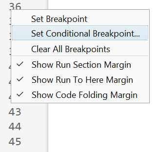
How to set a conditional break point
1. Right click the line number where you want the condition to be evaluated and select "Set Conditional Breakpoint"
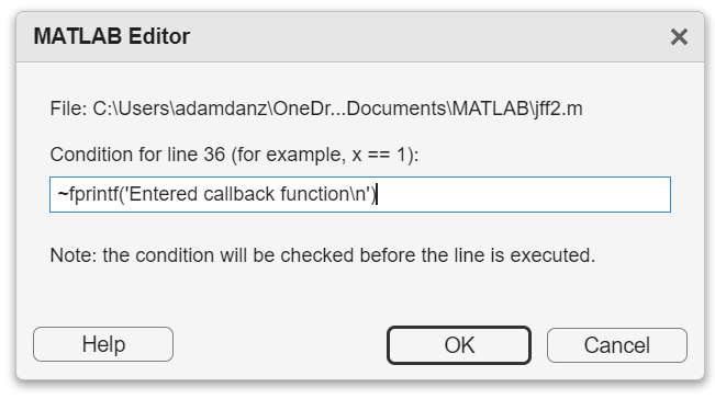
2. Enter a valid MATLAB expression that returns a logical scalar value in the editor dialog.
Handy one-liners
Check if a line is reached: Don't forget the negation (~) and the line break (\n)!
~fprintf('Entered callback function\n')
Display the call stack from the break point line: one of my favorites!
~fprintf('%s\n',formattedDisplayText(struct2table(dbstack)))
Inspect variable values: For scalar values,
~fprintf('v = %.5f\n', v)
~fprintf('%s\n', formattedDisplayText(v)).
Make sense of frequent hits: In some situations such as responses to listeners or interactive callbacks, a line can be executed 100s of times per second. Incorporate a timestamp to differentiate messages during rapid execution.
~fprintf('WindowButtonDownFcn - %s\n', datetime('now'))
Closing
This tip not only keeps your code clean but also offers a dynamic way to monitor code execution and variable states without permanent modifications. Interested in digging deeper? @Steve Eddins takes this tip to the next level with his Code Trace for MATLAB tool available on the File Exchange (read more).
Summary animation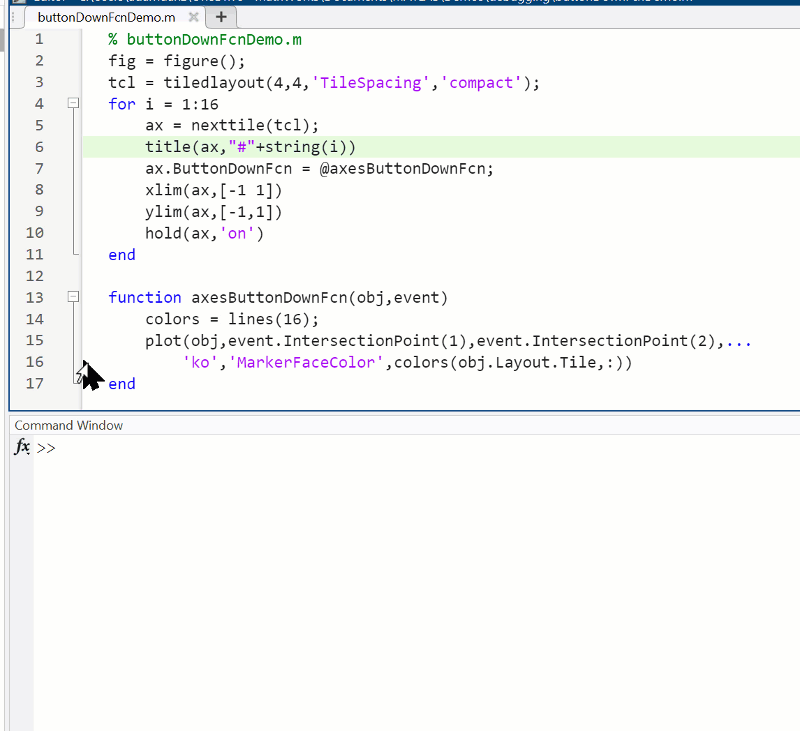
To reproduce the events in this animation:
% buttonDownFcnDemo.m
fig = figure();
tcl = tiledlayout(4,4,'TileSpacing','compact');
for i = 1:16
ax = nexttile(tcl);
title(ax,"#"+string(i))
ax.ButtonDownFcn = @axesButtonDownFcn;
xlim(ax,[-1 1])
ylim(ax,[-1,1])
hold(ax,'on')
end
function axesButtonDownFcn(obj,event)
colors = lines(16);
plot(obj,event.IntersectionPoint(1),event.IntersectionPoint(2),...
'ko','MarkerFaceColor',colors(obj.Layout.Tile,:))
end
numel(v)
6%
length(v)
13%
width(v)
14%
nnz(v)
8%
size(v, 1)
27%
sum(v > 0)
31%
2537 个投票
As far as I know, the MATLAB Community (including Matlab Central and Mathworks' official GitHub repository) has always been a vibrant and diverse professional and amateur community of MATLAB users from various fields globally. Being a part of it myself, especially in recent years, I have not only benefited continuously from the community but also tried to give back by helping other users in need.
I am a senior MATLAB user from Shenzhen, China, and I have a deep passion for MATLAB, applying it in various scenarios. Due to the less than ideal job market in my current social environment, I am hoping to find a position for remote support work within the Matlab Community. I wonder if this is realistic. For instance, Mathworks has been open-sourcing many repositories in recent years, especially in the field of deep learning with typical applications across industries. I am eager to use the latest MATLAB features to implement state-of-the-art algorithms. Additionally, I occasionally contribute through GitHub issues and pull requests.
In conclusion, I am looking forward to the opportunity to formally join the Matlab Community in a remote support role, dedicating more energy to giving back to the community and making the world a better place! (If a Mathworks employer can contact me, all the better~)
We're thrilled to unveil a new feature in the MATLAB Central community: User Following.
Our community is so lucky to have many experienced MATLAB experts who generously share their knowledge and insights across different applications, including Answers, File Exchange, Discussions, Contests, or Blogs.
With the introduction of User Following feature, you can now easily track new content across different areas and engage in discussions with people you follow. Simply click the ‘Follow’ button located on their profile page to start.
Depending on your communication setting, you will receive notifications via email and/or view updates in your ‘Followed Activity’ feeds. To tailor your feed, select the ‘People’ filter and focus on activities from those you follow.

We strongly encourage you to take advantage of the User Following feature to foster learning and collaboration within our vibrant community.
Who will be the first person you choose to follow? Share your answer in the comments section below and let's inspire each other to explore new horizons together.
How long until the 'dumbest' models are smarter than your average person? Thanks for sharing this article @Adam Danz
ismissing( { [ ] } )
26%
ismissing( NaN )
18%
ismissing( NaT )
11%
ismissing( missing )
21%
ismissing( categorical(missing) )
9%
ismissing( { '' } ) % 2 apostrophes
16%
896 个投票
I created an ellipse visualizer in #MATLAB using App Designer! To read more about it, and how it ties to the recent total solar eclipse, check out my latest blog post:
Github Repo of the app (you can open it on MATLAB Online!):
Hey MATLAB Community! 🌟
As we continue to explore, learn, and innovate together, it's essential to take a moment to recognize the remarkable contributions that have sparked engaging discussions, solved perplexing problems, and shared insightful knowledge in the past two weeks. Let's dive into the highlights that have made our community even more vibrant and resourceful.
Interesting Questions
Burhan Burak brings up an intriguing issue faced when running certain code in MATLAB, seeking advice on how to refactor the code to eliminate a warning message. It's a great example of the practical challenges we often encounter
Jenni asks for guidance on improving linear models to fit data points more accurately. This question highlights the common hurdles in data analysis and model fitting, sparking a conversation on best practices and methodologies.
Popular Discussions
A thought-provoking question posed by goc3 that delves into the intricacies of MATLAB's logical operations. It's a great discussion starter that tests and expands our understanding of MATLAB's behavior.
Toshiaki Takeuchi shares an insightful visualization of the demand for MATLAB jobs across different regions, based on data from LinkedIn. This post not only provides a snapshot of the job market but also encourages members to discuss trends in MATLAB's use in the industry.
From the Blogs
Mike Croucher shares his excitement and insights on two long-awaited features finally making their way into MATLAB R2024a. His post reflects the passion and persistence of our community members in enhancing MATLAB's functionality.
In this informative post, Sivylla Paraskevopoulou offers practical tips for speeding up the training of deep learning models. It's a must-read for anyone looking to optimize their deep learning workflows.
A Heartfelt Thank You 🙏
To everyone who asked a question, started a discussion, or wrote a blog post: Thank you! Your contributions are what make our community a fountain of knowledge, inspiration, and innovation. Let's keep the momentum going and continue to support each other in our journey to explore the vast universe of MATLAB.
Happy Coding!
Note: If you haven't yet, make sure to check out these highlights and add your voice to our growing community. Your insights and experiences are what make us stronger.
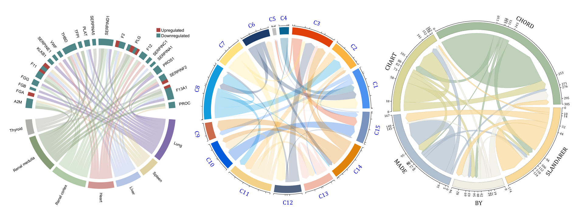
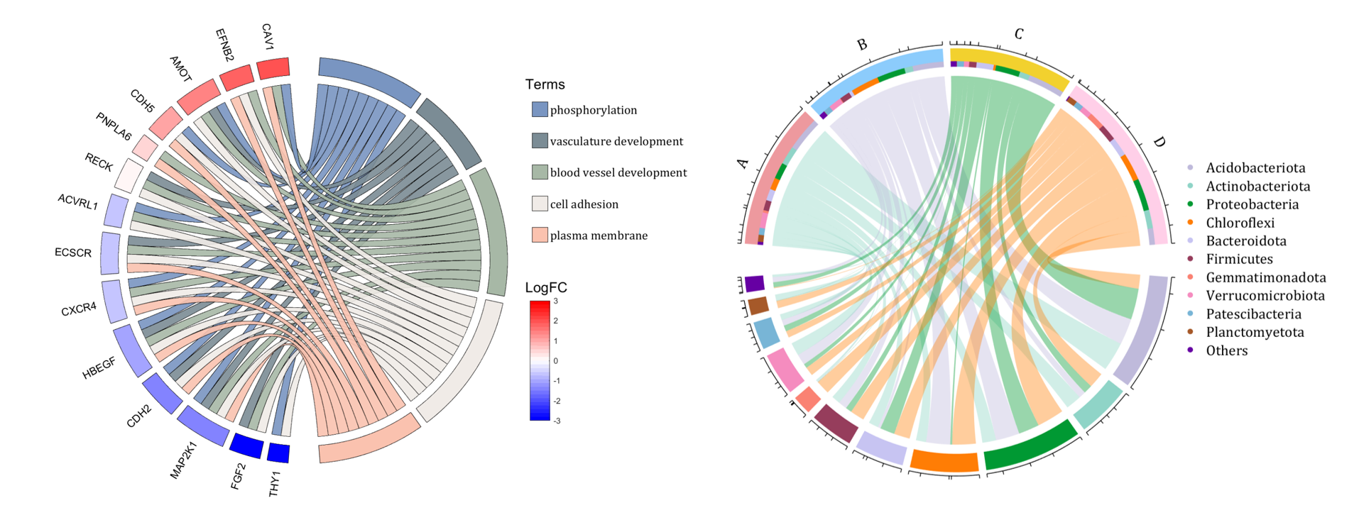
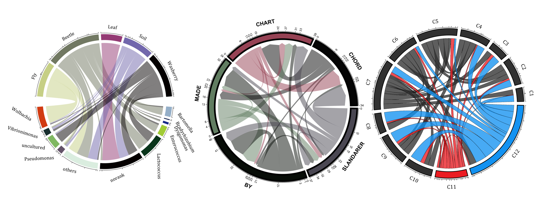
The beautiful and elegant chord diagrams were all created using MATLAB?
Indeed, they were all generated using the chord diagram plotting toolkit that I developed myself:
- - Chord chart: [chord chart](https://www.mathworks.com/matlabcentral/fileexchange/116550-chord-chart)
- - Directed graph chord chart: [digraph chord chart]:(https://www.mathworks.com/matlabcentral/fileexchange/121043-digraph-chord-chart)
You can download these toolkits from the provided links.
The reason for writing this article is that many people have started using the chord diagram plotting toolkit that I developed. However, some users are unsure about customizing certain styles. As the developer, I have a good understanding of the implementation principles of the toolkit and can apply it flexibly. This has sparked the idea of challenging myself to create various styles of chord diagrams. Currently, the existing code is quite lengthy. In the future, I may integrate some of this code into the toolkit, enabling users to achieve the effects of many lines of code with just a few lines.
Without further ado, let's see the extent to which this MATLAB toolkit can currently perform.
demo 1
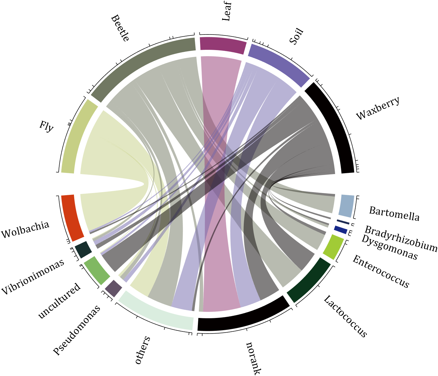
rng(2)
dataMat = randi([0,5], [11,5]);
dataMat(1:6,1) = 0;
dataMat([11,7],1) = [45,25];
dataMat([1,4,5,7],2) = [20,20,30,30];
dataMat(:,3) = 0;
dataMat(6,3) = 45;
dataMat(1:5,4) = 0;
dataMat([6,7],4) = [25,25];
dataMat([5,6,9],5) = [25,25,25];
colName = {'Fly', 'Beetle', 'Leaf', 'Soil', 'Waxberry'};
rowName = {'Bartomella', 'Bradyrhizobium', 'Dysgomonas', 'Enterococcus',...
'Lactococcus', 'norank', 'others', 'Pseudomonas', 'uncultured',...
'Vibrionimonas', 'Wolbachia'};
figure('Units','normalized', 'Position',[.02,.05,.6,.85])
CC = chordChart(dataMat, 'rowName',rowName, 'colName',colName, 'Sep',1/80);
CC = CC.draw();
% 修改上方方块颜色(Modify the color of the blocks above)
CListT = [0.7765 0.8118 0.5216; 0.4431 0.4706 0.3843; 0.5804 0.2275 0.4549;
0.4471 0.4039 0.6745; 0.0157 0 0 ];
for i = 1:size(dataMat, 2)
CC.setSquareT_N(i, 'FaceColor',CListT(i,:))
end
% 修改下方方块颜色(Modify the color of the blocks below)
CListF = [0.5843 0.6863 0.7843; 0.1098 0.1647 0.3255; 0.0902 0.1608 0.5373;
0.6314 0.7961 0.2118; 0.0392 0.2078 0.1059; 0.0157 0 0 ;
0.8549 0.9294 0.8745; 0.3882 0.3255 0.4078; 0.5020 0.7216 0.3843;
0.0902 0.1843 0.1804; 0.8196 0.2314 0.0706];
for i = 1:size(dataMat, 1)
CC.setSquareF_N(i, 'FaceColor',CListF(i,:))
end
% 修改弦颜色(Modify chord color)
for i = 1:size(dataMat, 1)
for j = 1:size(dataMat, 2)
CC.setChordMN(i,j, 'FaceColor',CListT(j,:), 'FaceAlpha',.5)
end
end
CC.tickState('on')
CC.labelRotate('on')
CC.setFont('FontSize',17, 'FontName','Cambria')
% CC.labelRotate('off')
% textHdl = findobj(gca,'Tag','ChordLabel');
% for i = 1:length(textHdl)
% if textHdl(i).Position(2) < 0
% if abs(textHdl(i).Position(1)) > .7
% textHdl(i).Rotation = textHdl(i).Rotation + 45;
% textHdl(i).HorizontalAlignment = 'right';
% if textHdl(i).Rotation > 90
% textHdl(i).Rotation = textHdl(i).Rotation + 180;
% textHdl(i).HorizontalAlignment = 'left';
% end
% else
% textHdl(i).Rotation = textHdl(i).Rotation + 10;
% textHdl(i).HorizontalAlignment = 'right';
% end
% end
% end
demo 2
rng(3)
dataMat = randi([1,15], [7,22]);
dataMat(dataMat < 11) = 0;
dataMat(1, sum(dataMat, 1) == 0) = 15;
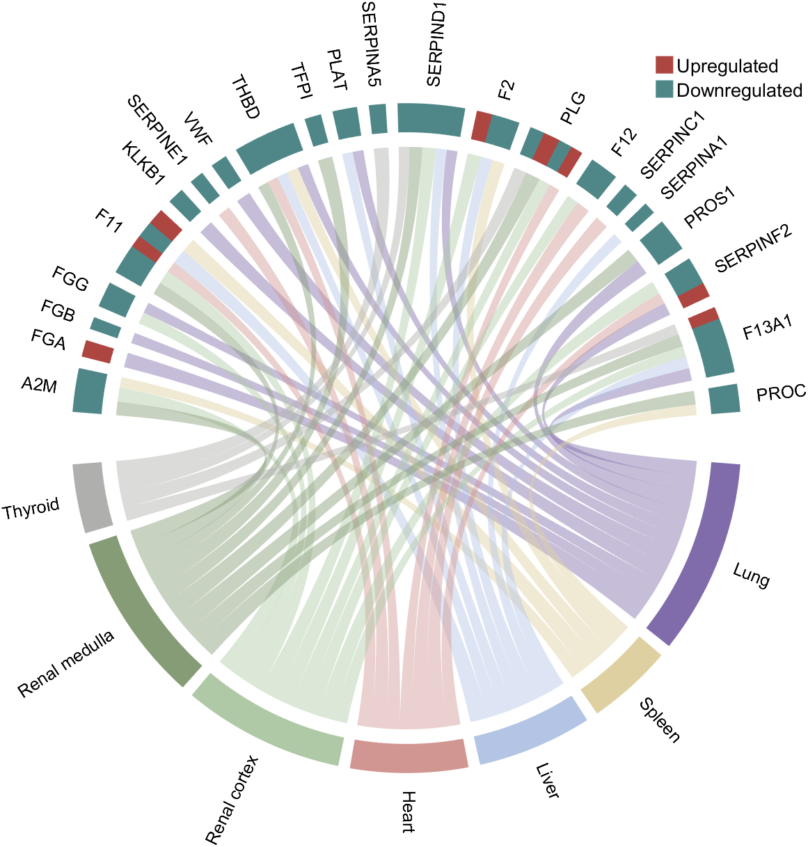
colName = {'A2M', 'FGA', 'FGB', 'FGG', 'F11', 'KLKB1', 'SERPINE1', 'VWF',...
'THBD', 'TFPI', 'PLAT', 'SERPINA5', 'SERPIND1', 'F2', 'PLG', 'F12',...
'SERPINC1', 'SERPINA1', 'PROS1', 'SERPINF2', 'F13A1', 'PROC'};
rowName = {'Lung', 'Spleen', 'Liver', 'Heart',...
'Renal cortex', 'Renal medulla', 'Thyroid'};
figure('Units','normalized', 'Position',[.02,.05,.6,.85])
CC = chordChart(dataMat, 'rowName',rowName, 'colName',colName, 'Sep',1/80, 'LRadius',1.21);
CC = CC.draw();
CC.labelRotate('on')
% 单独设置每一个弦末端方块(Set individual end blocks for each chord)
% Use obj.setEachSquareF_Prop
% or obj.setEachSquareT_Prop
% F means from (blocks below)
% T means to (blocks above)
CListT = [173,70,65; 79,135,136]./255;
% Upregulated:1 | Downregulated:2
Regulated = rand([7, 22]);
Regulated = (Regulated < .8) + 1;
for i = 1:size(Regulated, 1)
for j = 1:size(Regulated, 2)
CC.setEachSquareT_Prop(i, j, 'FaceColor', CListT(Regulated(i,j),:))
end
end
% 绘制图例(Draw legend)
H1 = fill([0,1,0] + 100, [1,0,1] + 100, CListT(1,:), 'EdgeColor','none');
H2 = fill([0,1,0] + 100, [1,0,1] + 100, CListT(2,:), 'EdgeColor','none');
lgdHdl = legend([H1,H2], {'Upregulated','Downregulated'}, 'AutoUpdate','off', 'Location','best');
lgdHdl.ItemTokenSize = [12,12];
lgdHdl.Box = 'off';
lgdHdl.FontSize = 13;
% 修改下方方块颜色(Modify the color of the blocks below)
CListF = [128,108,171; 222,208,161; 180,196,229; 209,150,146; 175,201,166;
134,156,118; 175,175,173]./255;
for i = 1:size(dataMat, 1)
CC.setSquareF_N(i, 'FaceColor',CListF(i,:))
end
% 修改弦颜色(Modify chord color)
for i = 1:size(dataMat, 1)
for j = 1:size(dataMat, 2)
CC.setChordMN(i,j, 'FaceColor',CListF(i,:), 'FaceAlpha',.45)
end
end
demo 3
dataMat = rand([15,15]);
dataMat(dataMat > .15) = 0;
CList = [ 75,146,241; 252,180, 65; 224, 64, 10; 5,100,146; 191,191,191;
26, 59,105; 255,227,130; 18,156,221; 202,107, 75; 0, 92,219;
243,210,136; 80, 99,129; 241,185,168; 224,131, 10; 120,147,190]./255;
figure('Units','normalized', 'Position',[.02,.05,.6,.85])
BCC = biChordChart(dataMat, 'Arrow','on', 'CData',CList);
BCC = BCC.draw();
% 添加刻度
BCC.tickState('on')
% 修改字体,字号及颜色
BCC.setFont('FontName','Cambria', 'FontSize',17, 'Color',[0,0,.8])
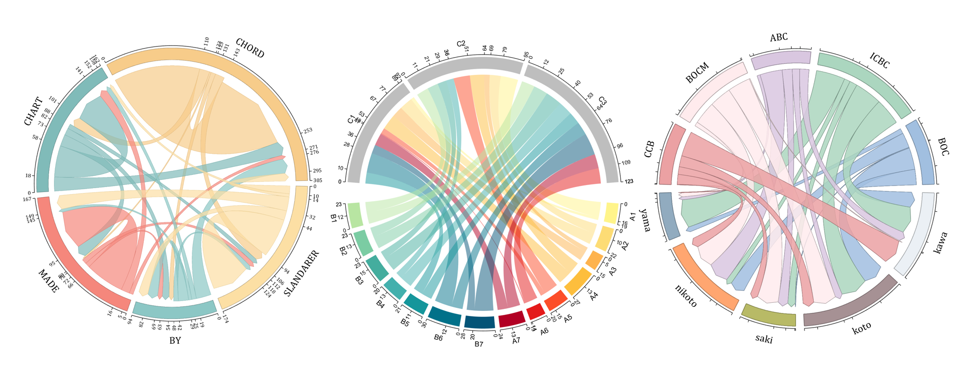
demo 4
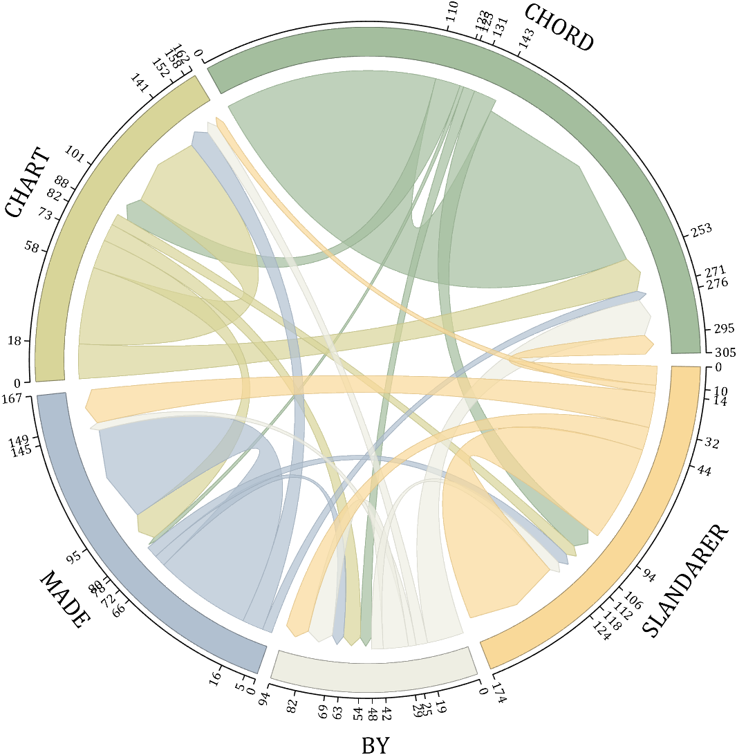
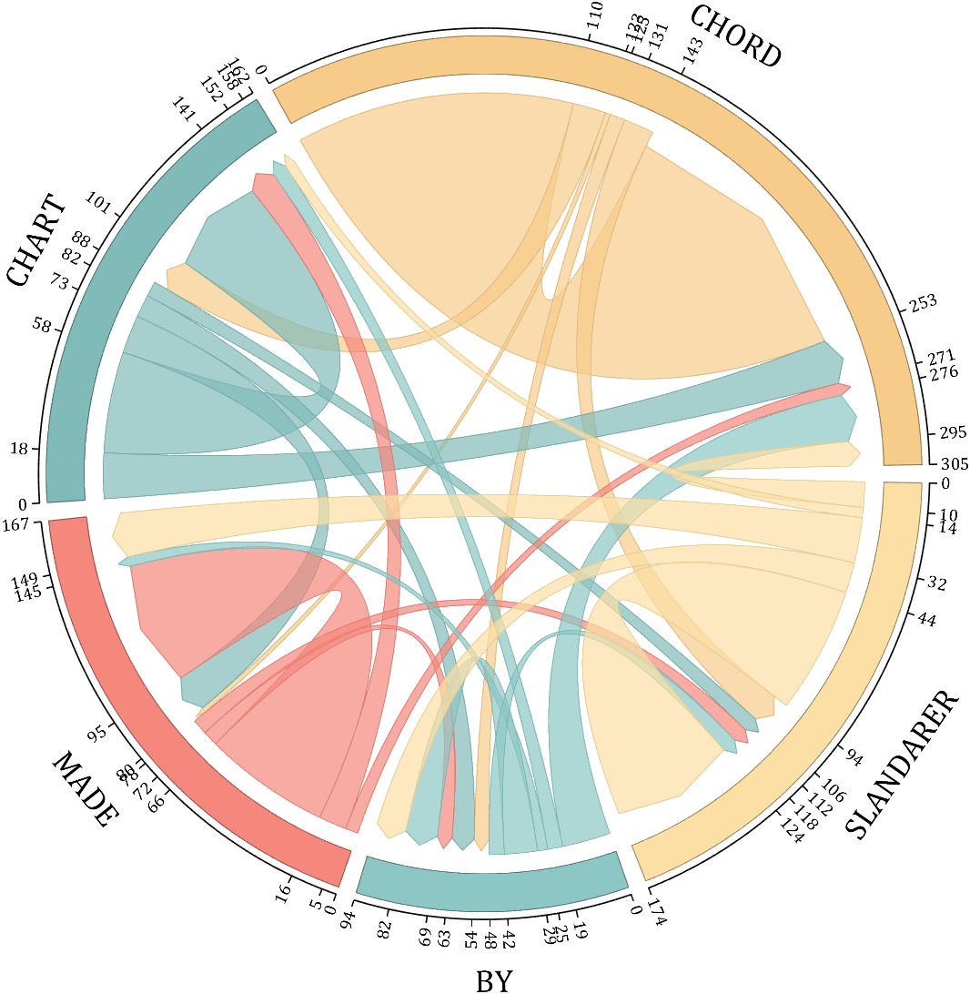
rng(5)
dataMat = randi([1,20], [5,5]);
dataMat(1,1) = 110;
dataMat(2,2) = 40;
dataMat(3,3) = 50;
dataMat(5,5) = 50;
CList1 = [164,190,158; 216,213,153; 177,192,208; 238,238,227; 249,217,153]./255;
CList2 = [247,204,138; 128,187,185; 245,135,124; 140,199,197; 252,223,164]./255;
CList = CList2;
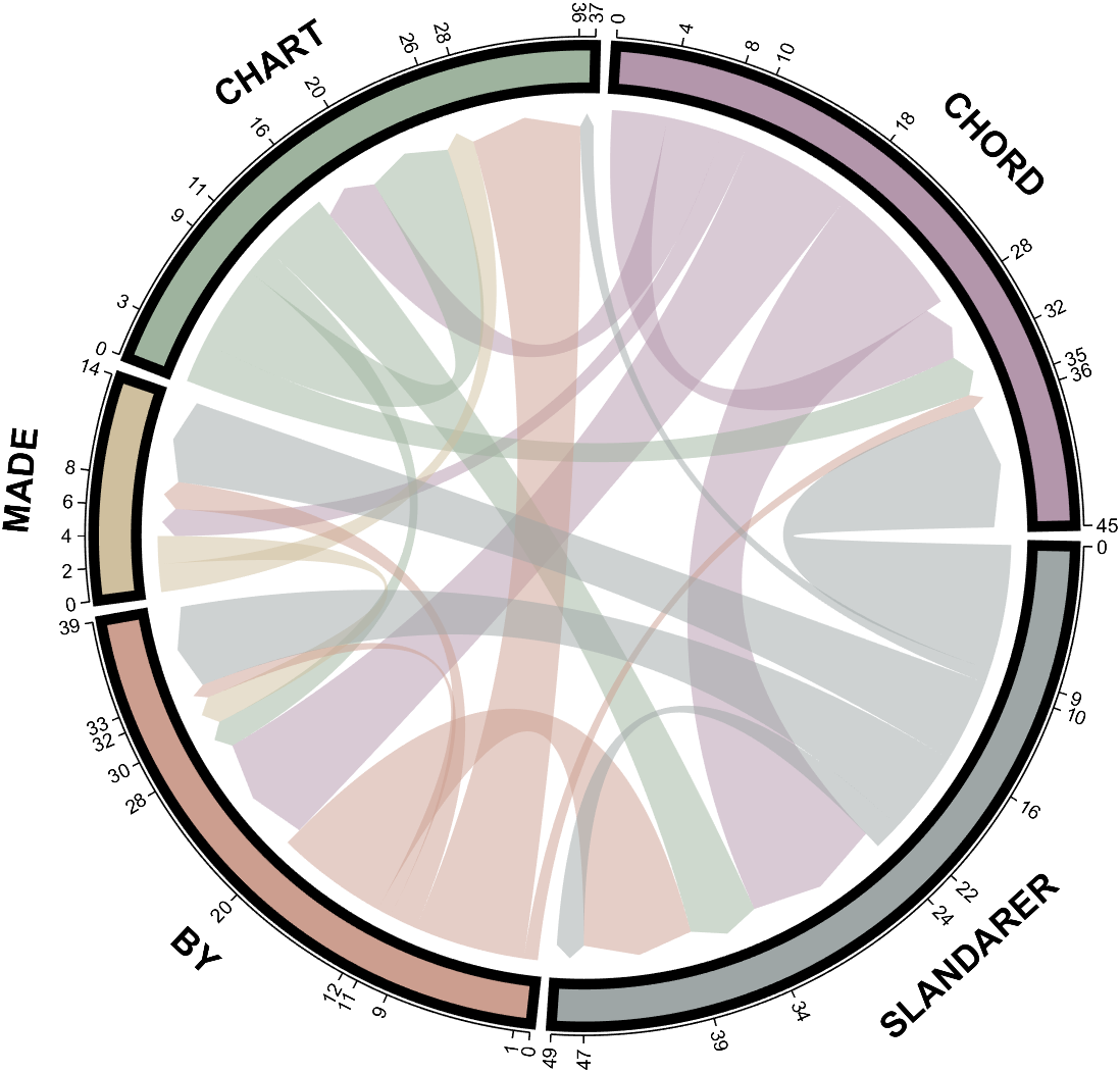
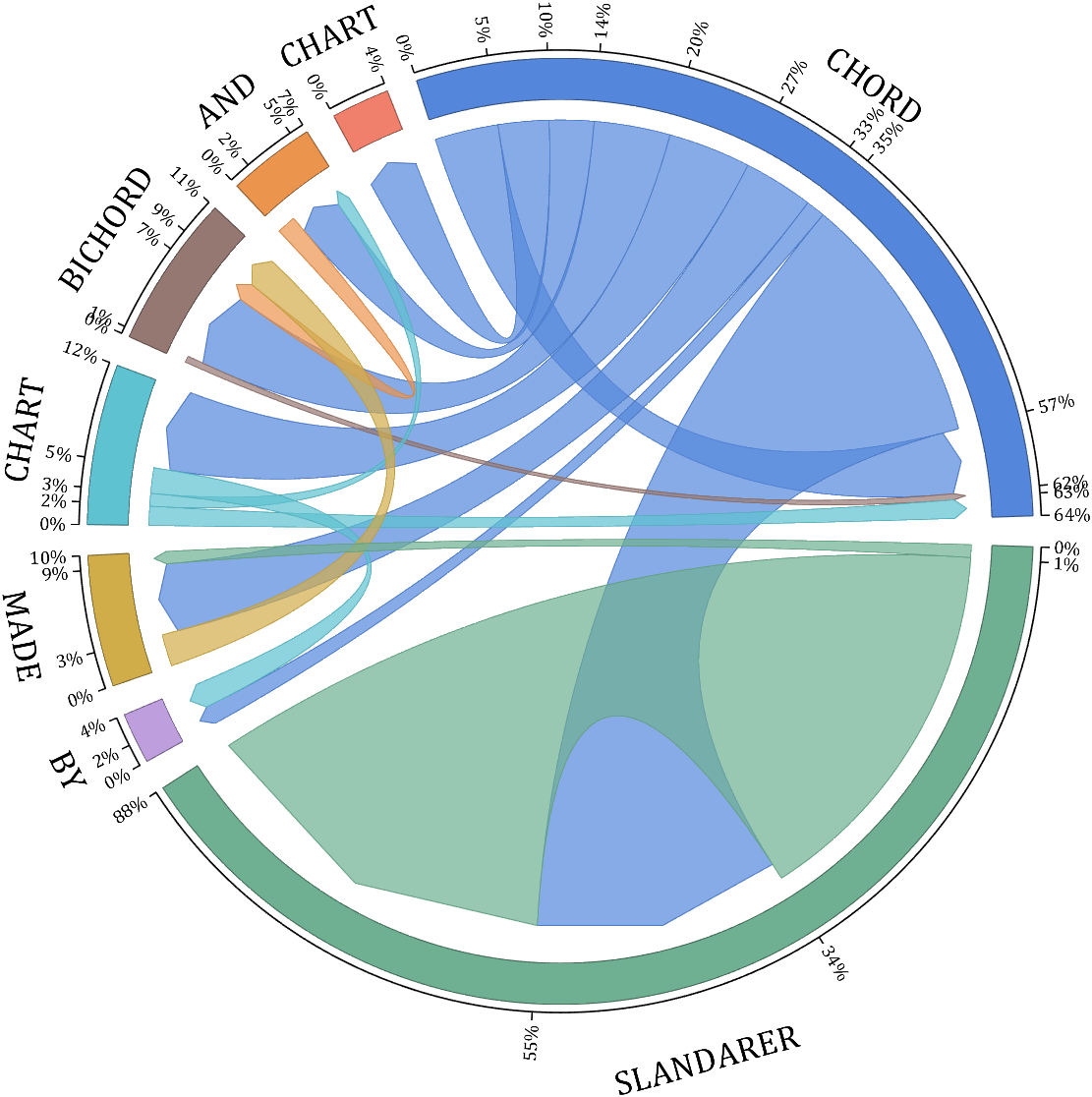
NameList={'CHORD','CHART','MADE','BY','SLANDARER'};
figure('Units','normalized', 'Position',[.02,.05,.6,.85])
BCC = biChordChart(dataMat, 'Arrow','on', 'CData',CList, 'Sep',1/30, 'Label',NameList, 'LRadius',1.33);
BCC = BCC.draw();
% 添加刻度
BCC.tickState('on')
% 修改弦颜色(Modify chord color)
for i = 1:size(dataMat, 1)
for j = 1:size(dataMat, 2)
if dataMat(i,j) > 0
BCC.setChordMN(i,j, 'FaceAlpha',.7, 'EdgeColor',CList(i,:)./1.1)
end
end
end
% 修改方块颜色(Modify the color of the blocks)
for i = 1:size(dataMat, 1)
BCC.setSquareN(i, 'EdgeColor',CList(i,:)./1.7)
end
% 修改字体,字号及颜色
BCC.setFont('FontName','Cambria', 'FontSize',17)
BCC.tickLabelState('on')
BCC.setTickFont('FontName','Cambria', 'FontSize',9)
demo 5
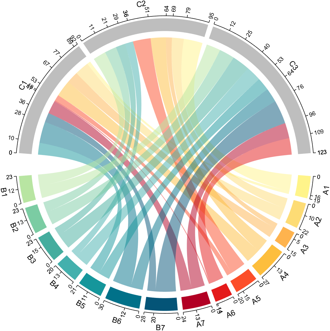
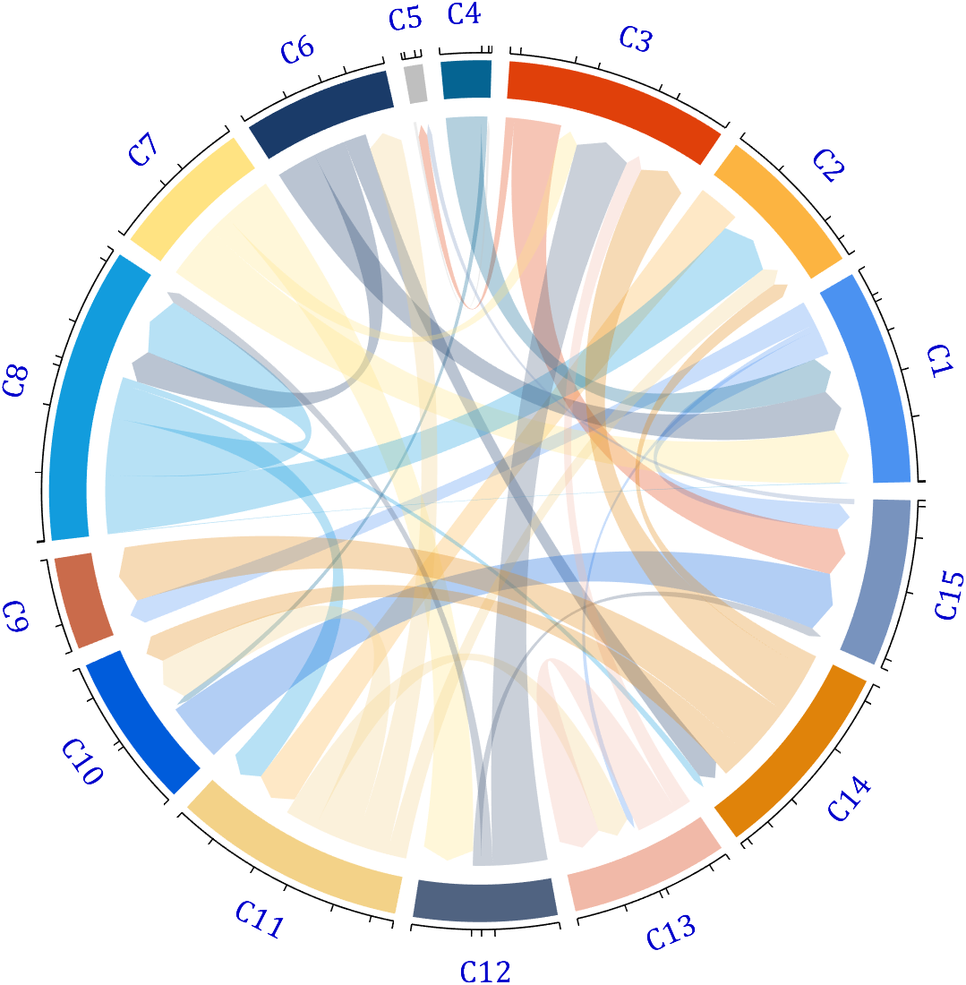
dataMat=randi([1,20], [14,3]);
dataMat(11:14,1) = 0;
dataMat(6:10,2) = 0;
dataMat(1:5,3) = 0;
colName = compose('C%d', 1:3);
rowName = [compose('A%d', 1:7), compose('B%d', 7:-1:1)];
figure('Units','normalized', 'Position',[.02,.05,.6,.85])
CC = chordChart(dataMat, 'rowName',rowName, 'colName',colName, 'Sep',1/80);
CC = CC.draw();
% 修改上方方块颜色(Modify the color of the blocks above)
for i = 1:size(dataMat, 2)
CC.setSquareT_N(i, 'FaceColor',[190,190,190]./255)
end
% 修改下方方块颜色(Modify the color of the blocks below)
CListF=[255,244,138; 253,220,117; 254,179, 78; 253,190, 61;
252, 78, 41; 228, 26, 26; 178, 0, 36; 4, 84,119;
1,113,137; 21,150,155; 67,176,173; 68,173,158;
123,204,163; 184,229,162]./255;
for i = 1:size(dataMat, 1)
CC.setSquareF_N(i, 'FaceColor',CListF(i,:))
end
% 修改弦颜色(Modify chord color)
for i = 1:size(dataMat, 1)
for j = 1:size(dataMat, 2)
CC.setChordMN(i,j, 'FaceColor',CListF(i,:), 'FaceAlpha',.5)
end
end
CC.tickState('on')
CC.tickLabelState('on')
demo 6
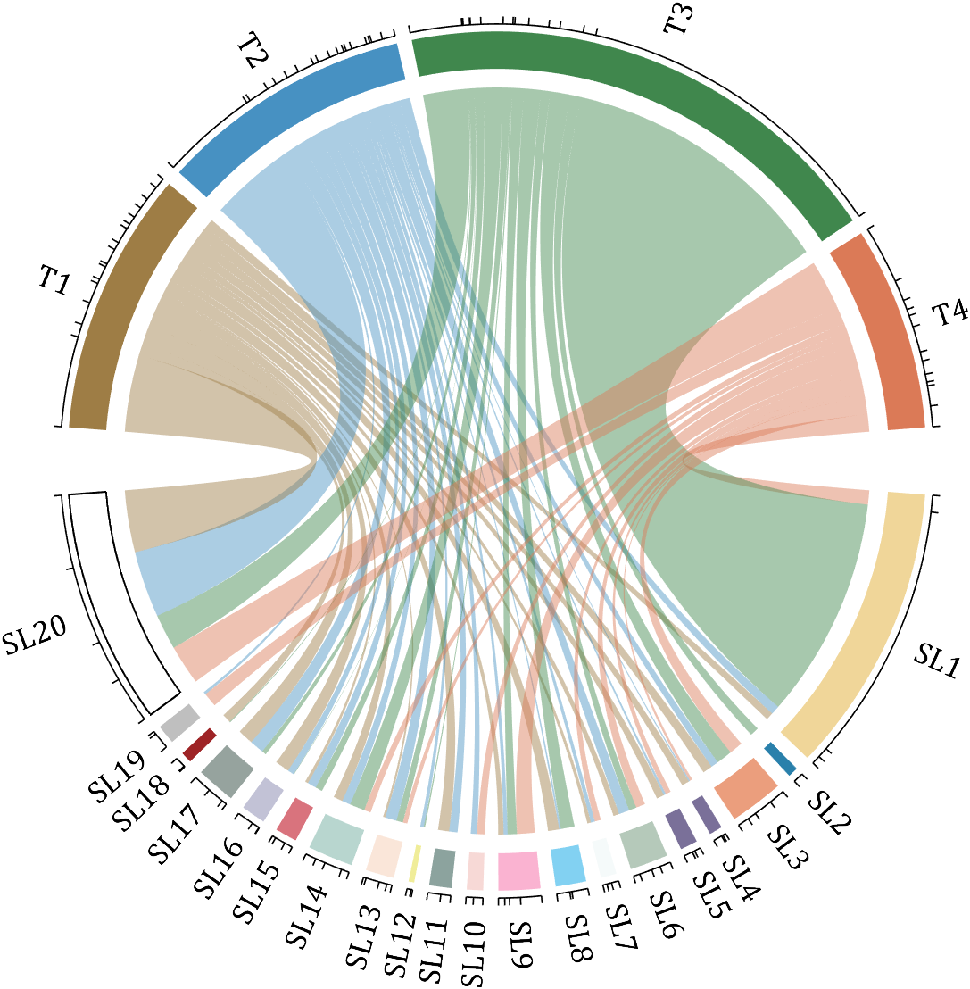
rng(2)
dataMat = randi([0,40], [20,4]);
dataMat(rand([20,4]) < .2) = 0;
dataMat(1,3) = 500;
dataMat(20,1:4) = [140; 150; 80; 90];
colName = compose('T%d', 1:4);
rowName = compose('SL%d', 1:20);
figure('Units','normalized', 'Position',[.02,.05,.6,.85])
CC = chordChart(dataMat, 'rowName',rowName, 'colName',colName, 'Sep',1/80, 'LRadius',1.23);
CC = CC.draw();
% 修改上方方块颜色(Modify the color of the blocks above)
CListT = [0.62,0.49,0.27; 0.28,0.57,0.76
0.25,0.53,0.30; 0.86,0.48,0.34];
for i = 1:size(dataMat, 2)
CC.setSquareT_N(i, 'FaceColor',CListT(i,:))
end
% 修改下方方块颜色(Modify the color of the blocks below)
CListF = [0.94,0.84,0.60; 0.16,0.50,0.67; 0.92,0.62,0.49;
0.48,0.44,0.60; 0.48,0.44,0.60; 0.71,0.79,0.73;
0.96,0.98,0.98; 0.51,0.82,0.95; 0.98,0.70,0.82;
0.97,0.85,0.84; 0.55,0.64,0.62; 0.94,0.93,0.60;
0.98,0.90,0.85; 0.72,0.84,0.81; 0.85,0.45,0.49;
0.76,0.76,0.84; 0.59,0.64,0.62; 0.62,0.14,0.15;
0.75,0.75,0.75; 1.00,1.00,1.00];
for i = 1:size(dataMat, 1)
CC.setSquareF_N(i, 'FaceColor',CListF(i,:))
end
CC.setSquareF_N(size(dataMat, 1), 'EdgeColor','k', 'LineWidth',1)
% 修改弦颜色(Modify chord color)
for i = 1:size(dataMat, 1)
for j = 1:size(dataMat, 2)
CC.setChordMN(i,j, 'FaceColor',CListT(j,:), 'FaceAlpha',.46)
end
end
CC.tickState('on')
CC.labelRotate('on')
CC.setFont('FontSize',17, 'FontName','Cambria')
demo 7
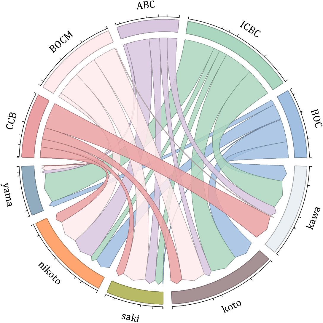
dataMat = randi([10,10000], [10,10]);
dataMat(6:10,:) = 0;
dataMat(:,1:5) = 0;
NameList = {'BOC', 'ICBC', 'ABC', 'BOCM', 'CCB', ...
'yama', 'nikoto', 'saki', 'koto', 'kawa'};
CList = [0.63,0.75,0.88
0.67,0.84,0.75
0.85,0.78,0.88
1.00,0.92,0.93
0.92,0.63,0.64
0.57,0.67,0.75
1.00,0.65,0.44
0.72,0.73,0.40
0.65,0.57,0.58
0.92,0.94,0.96];
figure('Units','normalized', 'Position',[.02,.05,.6,.85])
BCC = biChordChart(dataMat, 'Arrow','on', 'CData',CList, 'Label',NameList);
BCC = BCC.draw();
% 修改弦颜色(Modify chord color)
for i = 1:size(dataMat, 1)
for j = 1:size(dataMat, 2)
if dataMat(i,j) > 0
BCC.setChordMN(i,j, 'FaceAlpha',.85, 'EdgeColor',CList(i,:)./1.5, 'LineWidth',.8)
end
end
end
for i = 1:size(dataMat, 1)
BCC.setSquareN(i, 'EdgeColor',CList(i,:)./1.5, 'LineWidth',1)
end
% 添加刻度、修改字体
BCC.tickState('on')
BCC.setFont('FontName','Cambria', 'FontSize',17)
demo 8
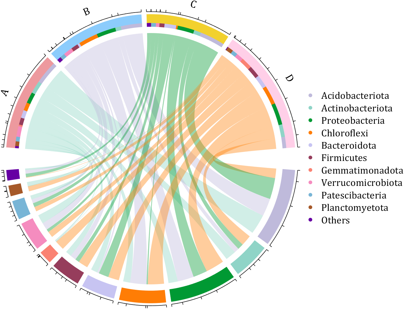
dataMat = rand([11,4]);
dataMat = round(10.*dataMat.*((11:-1:1).'+1))./10;
colName = {'A','B','C','D'};
rowName = {'Acidobacteriota', 'Actinobacteriota', 'Proteobacteria', ...
'Chloroflexi', 'Bacteroidota', 'Firmicutes', 'Gemmatimonadota', ...
'Verrucomicrobiota', 'Patescibacteria', 'Planctomyetota', 'Others'};
figure('Units','normalized', 'Position',[.02,.05,.8,.85])
CC = chordChart(dataMat, 'colName',colName, 'Sep',1/80, 'SSqRatio',30/100);% -30/100
CC = CC.draw();
% 修改上方方块颜色(Modify the color of the blocks above)
CListT = [0.93,0.60,0.62
0.55,0.80,0.99
0.95,0.82,0.18
1.00,0.81,0.91];
for i = 1:size(dataMat, 2)
CC.setSquareT_N(i, 'FaceColor',CListT(i,:))
end
% 修改下方方块颜色(Modify the color of the blocks below)
CListF = [0.75,0.73,0.86
0.56,0.83,0.78
0.00,0.60,0.20
1.00,0.49,0.02
0.78,0.77,0.95
0.59,0.24,0.36
0.98,0.51,0.45
0.96,0.55,0.75
0.47,0.71,0.84
0.65,0.35,0.16
0.40,0.00,0.64];
for i = 1:size(dataMat, 1)
CC.setSquareF_N(i, 'FaceColor',CListF(i,:))
end
% 修改弦颜色(Modify chord color)
CListC = [0.55,0.83,0.76
0.75,0.73,0.86
0.00,0.60,0.19
1.00,0.51,0.04];
for i = 1:size(dataMat, 1)
for j = 1:size(dataMat, 2)
CC.setChordMN(i,j, 'FaceColor',CListC(j,:), 'FaceAlpha',.4)
end
end
% 单独设置每一个弦末端方块(Set individual end blocks for each chord)
% Use obj.setEachSquareF_Prop
% or obj.setEachSquareT_Prop
% F means from (blocks below)
% T means to (blocks above)
for i = 1:size(dataMat, 1)
for j = 1:size(dataMat, 2)
CC.setEachSquareT_Prop(i,j, 'FaceColor', CListF(i,:))
end
end
% 添加刻度
CC.tickState('on')
% 修改字体,字号及颜色
CC.setFont('FontName','Cambria', 'FontSize',17)
% 隐藏下方标签
textHdl = findobj(gca, 'Tag','ChordLabel');
for i = 1:length(textHdl)
if textHdl(i).Position(2) < 0
set(textHdl(i), 'Visible','off')
end
end
% 绘制图例(Draw legend)
scatterHdl = scatter(10.*ones(size(dataMat,1)),10.*ones(size(dataMat,1)), ...
55, 'filled');
for i = 1:length(scatterHdl)
scatterHdl(i).CData = CListF(i,:);
end
lgdHdl = legend(scatterHdl, rowName, 'Location','best', 'FontSize',16, 'FontName','Cambria', 'Box','off');
set(lgdHdl, 'Position',[.7482,.3577,.1658,.3254])
demo 9
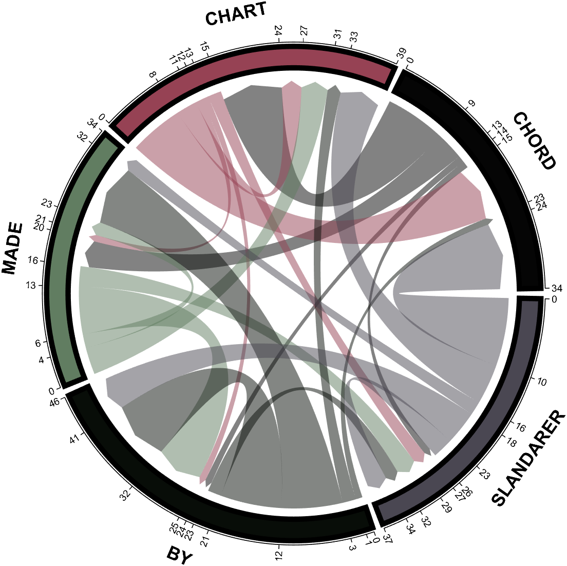
dataMat = randi([0,10], [5,5]);
CList1 = [0.70,0.59,0.67
0.62,0.70,0.62
0.81,0.75,0.62
0.80,0.62,0.56
0.62,0.65,0.65];
CList2 = [0.02,0.02,0.02
0.59,0.26,0.33
0.38,0.49,0.38
0.03,0.05,0.03
0.29,0.28,0.32];
CList = CList2;
NameList={'CHORD','CHART','MADE','BY','SLANDARER'};
figure('Units','normalized', 'Position',[.02,.05,.6,.85])
BCC = biChordChart(dataMat, 'Arrow','on', 'CData',CList, 'Sep',1/30, 'Label',NameList, 'LRadius',1.33);
BCC = BCC.draw();
% 修改弦颜色(Modify chord color)
for i = 1:size(dataMat, 1)
for j = 1:size(dataMat, 2)
BCC.setChordMN(i,j, 'FaceAlpha',.5)
end
end
% 修改方块颜色(Modify the color of the blocks)
for i = 1:size(dataMat, 1)
BCC.setSquareN(i, 'EdgeColor',[0,0,0], 'LineWidth',5)
end
% 添加刻度
BCC.tickState('on')
% 修改字体,字号及颜色
BCC.setFont('FontSize',17, 'FontWeight','bold')
BCC.tickLabelState('on')
BCC.setTickFont('FontSize',9)
demo 10
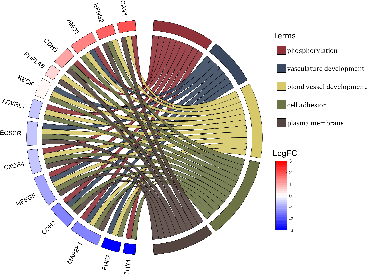
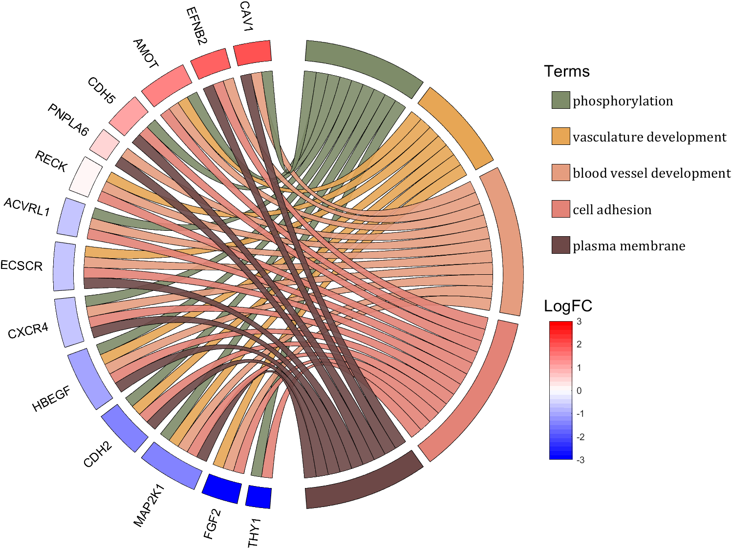
rng(2)
dataMat = rand([14,5]) > .3;
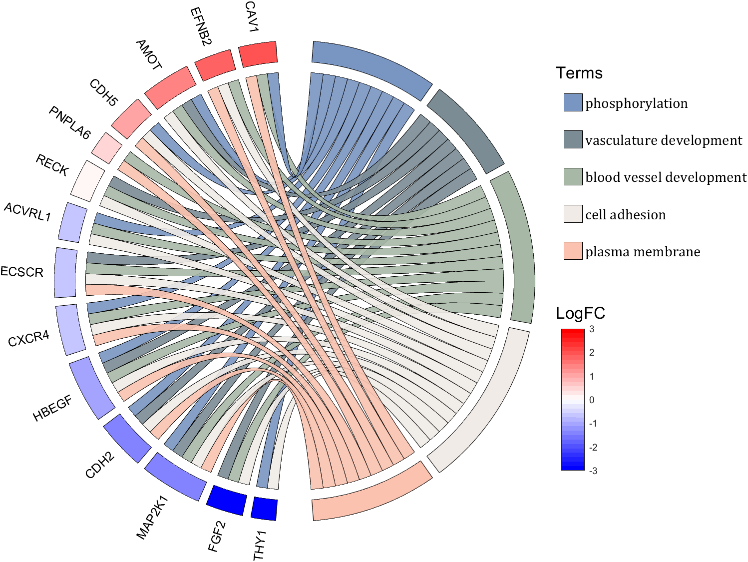
colName = {'phosphorylation', 'vasculature development', 'blood vessel development', ...
'cell adhesion', 'plasma membrane'};
rowName = {'THY1', 'FGF2', 'MAP2K1', 'CDH2', 'HBEGF', 'CXCR4', 'ECSCR',...
'ACVRL1', 'RECK', 'PNPLA6', 'CDH5', 'AMOT', 'EFNB2', 'CAV1'};
figure('Units','normalized', 'Position',[.02,.05,.9,.85])
CC = chordChart(dataMat, 'colName',colName, 'rowName',rowName, 'Sep',1/80, 'LRadius',1.2);
CC = CC.draw();
% 修改上方方块颜色(Modify the color of the blocks above)
CListT1 = [0.5686 0.1961 0.2275
0.2275 0.2863 0.3765
0.8431 0.7882 0.4118
0.4275 0.4510 0.2706
0.3333 0.2706 0.2510];
CListT2 = [0.4941 0.5490 0.4118
0.9059 0.6510 0.3333
0.8980 0.6157 0.4980
0.8902 0.5137 0.4667
0.4275 0.2824 0.2784];
CListT3 = [0.4745 0.5843 0.7569
0.4824 0.5490 0.5843
0.6549 0.7216 0.6510
0.9412 0.9216 0.9059
0.9804 0.7608 0.6863];
CListT = CListT3;
for i = 1:size(dataMat, 2)
CC.setSquareT_N(i, 'FaceColor',CListT(i,:), 'EdgeColor',[0,0,0])
end
% 修改弦颜色(Modify chord color)
for i = 1:size(dataMat, 1)
for j = 1:size(dataMat, 2)
CC.setChordMN(i,j, 'FaceColor',CListT(j,:), 'FaceAlpha',.9, 'EdgeColor',[0,0,0])
end
end
% 修改下方方块颜色(Modify the color of the blocks below)
logFC = sort(rand(1,14))*6 - 3;
for i = 1:size(dataMat, 1)
CC.setSquareF_N(i, 'CData',logFC(i), 'FaceColor','flat', 'EdgeColor',[0,0,0])
end
CMap = [ 0 0 1.0000; 0.0645 0.0645 1.0000; 0.1290 0.1290 1.0000; 0.1935 0.1935 1.0000
0.2581 0.2581 1.0000; 0.3226 0.3226 1.0000; 0.3871 0.3871 1.0000; 0.4516 0.4516 1.0000
0.5161 0.5161 1.0000; 0.5806 0.5806 1.0000; 0.6452 0.6452 1.0000; 0.7097 0.7097 1.0000
0.7742 0.7742 1.0000; 0.8387 0.8387 1.0000; 0.9032 0.9032 1.0000; 0.9677 0.9677 1.0000
1.0000 0.9677 0.9677; 1.0000 0.9032 0.9032; 1.0000 0.8387 0.8387; 1.0000 0.7742 0.7742
1.0000 0.7097 0.7097; 1.0000 0.6452 0.6452; 1.0000 0.5806 0.5806; 1.0000 0.5161 0.5161
1.0000 0.4516 0.4516; 1.0000 0.3871 0.3871; 1.0000 0.3226 0.3226; 1.0000 0.2581 0.2581
1.0000 0.1935 0.1935; 1.0000 0.1290 0.1290; 1.0000 0.0645 0.0645; 1.0000 0 0];
colormap(CMap);
try clim([-3,3]),catch,end
try caxis([-3,3]),catch,end
CBHdl = colorbar();
CBHdl.Position = [0.74,0.25,0.02,0.2];
% =========================================================================
% 交换XY轴(Swap XY axis)
patchHdl = findobj(gca, 'Type','patch');
for i = 1:length(patchHdl)
tX = patchHdl(i).XData;
tY = patchHdl(i).YData;
patchHdl(i).XData = tY;
patchHdl(i).YData = - tX;
end
txtHdl = findobj(gca, 'Type','text');
for i = 1:length(txtHdl)
txtHdl(i).Position([1,2]) = [1,-1].*txtHdl(i).Position([2,1]);
if txtHdl(i).Position(1) < 0
txtHdl(i).HorizontalAlignment = 'right';
else
txtHdl(i).HorizontalAlignment = 'left';
end
end
lineHdl = findobj(gca, 'Type','line');
for i = 1:length(lineHdl)
tX = lineHdl(i).XData;
tY = lineHdl(i).YData;
lineHdl(i).XData = tY;
lineHdl(i).YData = - tX;
end
% =========================================================================
txtHdl = findobj(gca, 'Type','text');
for i = 1:length(txtHdl)
if txtHdl(i).Position(1) > 0
txtHdl(i).Visible = 'off';
end
end
text(1.25,-.15, 'LogFC', 'FontSize',16)
text(1.25,1, 'Terms', 'FontSize',16)
patchHdl = [];
for i = 1:size(dataMat, 2)
patchHdl(i) = fill([10,11,12],[10,13,13], CListT(i,:), 'EdgeColor',[0,0,0]);
end
lgdHdl = legend(patchHdl, colName, 'Location','best', 'FontSize',14, 'FontName','Cambria', 'Box','off');
lgdHdl.Position = [.735,.53,.167,.27];
lgdHdl.ItemTokenSize = [18,8];
demo 11
rng(2)
dataMat = rand([12,12]);
dataMat(dataMat < .85) = 0;
dataMat(7,:) = 1.*(rand(1,12)+.1);
dataMat(11,:) = .6.*(rand(1,12)+.1);
dataMat(12,:) = [2.*(rand(1,10)+.1), 0, 0];
CList = [repmat([49,49,49],[10,1]); 235,28,34; 19,146,241]./255;
figure('Units','normalized', 'Position',[.02,.05,.6,.85])
BCC = biChordChart(dataMat, 'Arrow','off', 'CData',CList);
BCC = BCC.draw();
% 添加刻度
BCC.tickState('on')
% 修改字体,字号及颜色
BCC.setFont('FontName','Cambria', 'FontSize',17)
% 修改弦颜色(Modify chord color)
for i = 1:size(dataMat, 1)
for j = 1:size(dataMat, 2)
if dataMat(i,j) > 0
BCC.setChordMN(i,j, 'FaceAlpha',.78, 'EdgeColor',[0,0,0])
end
end
end
% 修改方块颜色(Modify the color of the blocks)
for i = 1:size(dataMat, 1)
BCC.setSquareN(i, 'EdgeColor',[0,0,0], 'LineWidth',2)
end
demo 12
dataMat = rand([9,9]);
dataMat(dataMat > .7) = 0;
dataMat(eye(9) == 1) = (rand([1,9])+.2).*3;
CList = [0.85,0.23,0.24
0.96,0.39,0.18
0.98,0.63,0.22
0.99,0.80,0.26
0.70,0.76,0.21
0.24,0.74,0.71
0.27,0.65,0.84
0.09,0.37,0.80
0.64,0.40,0.84];
figure('Units','normalized', 'Position',[.02,.05,.6,.85])
BCC = biChordChart(dataMat, 'Arrow','on', 'CData',CList);
BCC = BCC.draw();
% 添加刻度、刻度标签
BCC.tickState('on')
% 修改字体,字号及颜色
BCC.setFont('FontName','Cambria', 'FontSize',17)
% 修改弦颜色(Modify chord color)
for i = 1:size(dataMat, 1)
for j = 1:size(dataMat, 2)
if dataMat(i,j) > 0
BCC.setChordMN(i,j, 'FaceAlpha',.7)
end
end
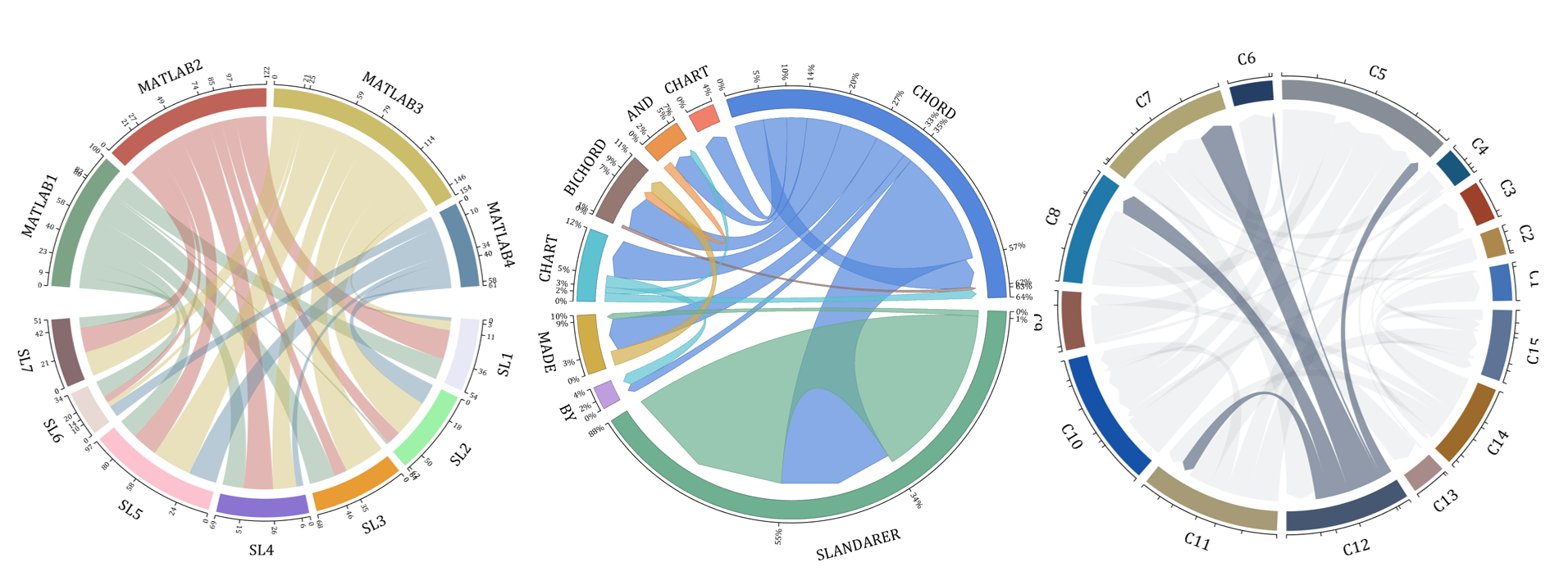
end
demo 13
rng(2)
dataMat = randi([1,40], [7,4]);
dataMat(rand([7,4]) < .1) = 0;
colName = compose('MATLAB%d', 1:4);
rowName = compose('SL%d', 1:7);
figure('Units','normalized', 'Position',[.02,.05,.7,.85])
CC = chordChart(dataMat, 'rowName',rowName, 'colName',colName, 'Sep',1/80, 'LRadius',1.32);
CC = CC.draw();
% 修改上方方块颜色(Modify the color of the blocks above)
CListT = [0.49,0.64,0.53
0.75,0.39,0.35
0.80,0.74,0.42
0.40,0.55,0.66];
for i = 1:size(dataMat, 2)
CC.setSquareT_N(i, 'FaceColor',CListT(i,:))
end
% 修改下方方块颜色(Modify the color of the blocks below)
CListF = [0.91,0.91,0.97
0.62,0.95,0.66
0.91,0.61,0.20
0.54,0.45,0.82
0.99,0.76,0.81
0.91,0.85,0.83
0.53,0.42,0.43];
for i = 1:size(dataMat, 1)
CC.setSquareF_N(i, 'FaceColor',CListF(i,:))
end
% 修改弦颜色(Modify chord color)
for i = 1:size(dataMat, 1)
for j = 1:size(dataMat, 2)
CC.setChordMN(i,j, 'FaceColor',CListT(j,:), 'FaceAlpha',.46)
end
end
CC.tickState('on')
CC.tickLabelState('on')
CC.setFont('FontSize',17, 'FontName','Cambria')
CC.setTickFont('FontSize',8, 'FontName','Cambria')
% 绘制图例(Draw legend)
scatterHdl = scatter(10.*ones(size(dataMat,1)),10.*ones(size(dataMat,1)), ...
55, 'filled');
for i = 1:length(scatterHdl)
scatterHdl(i).CData = CListF(i,:);
end
lgdHdl = legend(scatterHdl, rowName, 'Location','best', 'FontSize',16, 'FontName','Cambria', 'Box','off');
set(lgdHdl, 'Position',[.77,.38,.1658,.27])
demo 14
rng(6)
dataMat = randi([1,20], [8,8]);
dataMat(dataMat > 5) = 0;
dataMat(1,:) = randi([1,15], [1,8]);
dataMat(1,8) = 40;
dataMat(8,8) = 60;
dataMat = dataMat./sum(sum(dataMat));
CList = [0.33,0.53,0.86
0.94,0.50,0.42
0.92,0.58,0.30
0.59,0.47,0.45
0.37,0.76,0.82
0.82,0.68,0.29
0.75,0.62,0.87
0.43,0.69,0.57];
NameList={'CHORD', 'CHART', 'AND', 'BICHORD',...
'CHART', 'MADE', 'BY', 'SLANDARER'};
figure('Units','normalized', 'Position',[.02,.05,.6,.85])
BCC = biChordChart(dataMat, 'Arrow','on', 'CData',CList, 'Sep',1/12, 'Label',NameList, 'LRadius',1.33);
BCC = BCC.draw();
% 添加刻度
BCC.tickState('on')
% 修改弦颜色(Modify chord color)
for i = 1:size(dataMat, 1)
for j = 1:size(dataMat, 2)
if dataMat(i,j) > 0
BCC.setChordMN(i,j, 'FaceAlpha',.7, 'EdgeColor',CList(i,:)./1.1)
end
end
end
% 修改方块颜色(Modify the color of the blocks)
for i = 1:size(dataMat, 1)
BCC.setSquareN(i, 'EdgeColor',CList(i,:)./1.7)
end
% 修改字体,字号及颜色
BCC.setFont('FontName','Cambria', 'FontSize',17)
BCC.tickLabelState('on')
BCC.setTickFont('FontName','Cambria', 'FontSize',9)
% 调整数值字符串格式
% Adjust numeric string format
BCC.setTickLabelFormat(@(x)[num2str(round(x*100)),'%'])
demo 15
CList = [0.81,0.72,0.83
0.69,0.82,0.89
0.17,0.44,0.64
0.70,0.85,0.55
0.03,0.57,0.13
0.97,0.67,0.64
0.84,0.09,0.12
1.00,0.80,0.46
0.98,0.52,0.01
];
figure('Units','normalized', 'Position',[.02,.05,.53,.85], 'Color',[1,1,1])
% =========================================================================
ax1 = axes('Parent',gcf, 'Position',[0,1/2,1/2,1/2]);
dataMat = rand([9,9]);
dataMat(dataMat > .4) = 0;
BCC = biChordChart(dataMat, 'Arrow','on', 'CData',CList);
BCC = BCC.draw();
BCC.tickState('on')
BCC.setFont('Visible','off')
% 修改弦颜色(Modify chord color)
for i = 1:size(dataMat, 1)
for j = 1:size(dataMat, 2)
if dataMat(i,j) > 0
BCC.setChordMN(i,j, 'FaceAlpha',.6)
end
end
end
text(-1.2,1.2, 'a', 'FontName','Times New Roman', 'FontSize',35)
% =========================================================================
ax2 = axes('Parent',gcf, 'Position',[1/2,1/2,1/2,1/2]);
dataMat = rand([9,9]);
dataMat(dataMat > .4) = 0;
dataMat = dataMat.*(1:9);
BCC = biChordChart(dataMat, 'Arrow','on', 'CData',CList);
BCC = BCC.draw();
BCC.tickState('on')
BCC.setFont('Visible','off')
% 修改弦颜色(Modify chord color)
for i = 1:size(dataMat, 1)
for j = 1:size(dataMat, 2)
if dataMat(i,j) > 0
BCC.setChordMN(i,j, 'FaceAlpha',.6)
end
end
end
text(-1.2,1.2, 'b', 'FontName','Times New Roman', 'FontSize',35)
% =========================================================================
ax3 = axes('Parent',gcf, 'Position',[0,0,1/2,1/2]);
dataMat = rand([9,9]);
dataMat(dataMat > .4) = 0;
dataMat = dataMat.*(1:9).';
BCC = biChordChart(dataMat, 'Arrow','on', 'CData',CList);
BCC = BCC.draw();
BCC.tickState('on')
BCC.setFont('Visible','off')
% 修改弦颜色(Modify chord color)
for i = 1:size(dataMat, 1)
for j = 1:size(dataMat, 2)
if dataMat(i,j) > 0
BCC.setChordMN(i,j, 'FaceAlpha',.6)
end
end
end
text(-1.2,1.2, 'c', 'FontName','Times New Roman', 'FontSize',35)
% =========================================================================
ax4 = axes('Parent',gcf, 'Position',[1/2,0,1/2,1/2]);
ax4.XColor = 'none'; ax4.YColor = 'none';
ax4.XLim = [-1,1]; ax4.YLim = [-1,1];
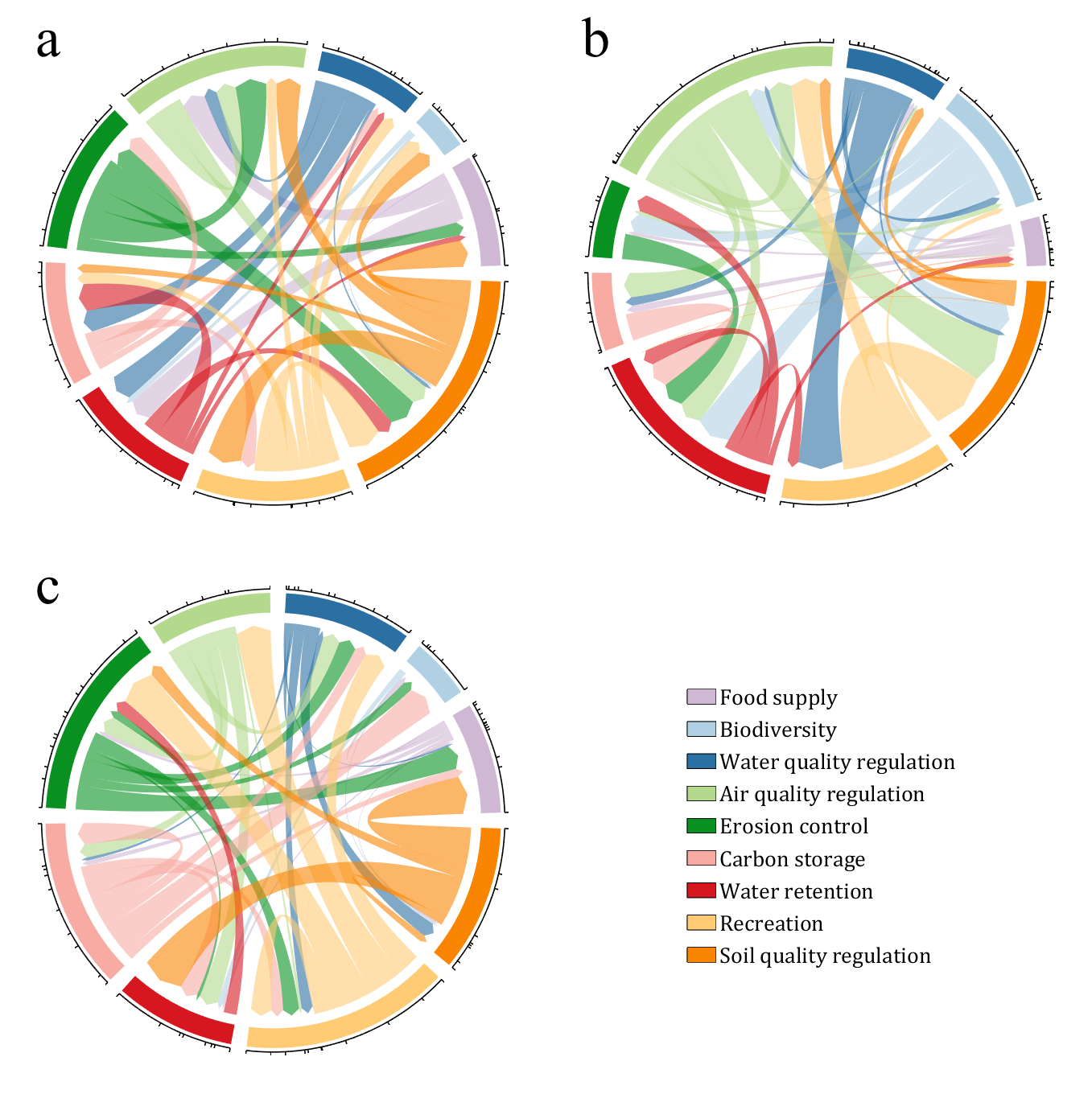
hold on
NameList = {'Food supply', 'Biodiversity', 'Water quality regulation', ...
'Air quality regulation', 'Erosion control', 'Carbon storage', ...
'Water retention', 'Recreation', 'Soil quality regulation'};
patchHdl = [];
for i = 1:size(dataMat, 2)
patchHdl(i) = fill([10,11,12],[10,13,13], CList(i,:), 'EdgeColor',[0,0,0]);
end
lgdHdl = legend(patchHdl, NameList, 'Location','best', 'FontSize',14, 'FontName','Cambria', 'Box','off');
lgdHdl.Position = [.625,.11,.255,.27];
lgdHdl.ItemTokenSize = [18,8];
demo 16
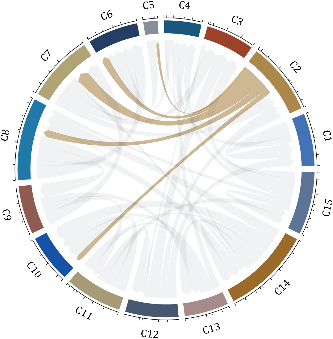
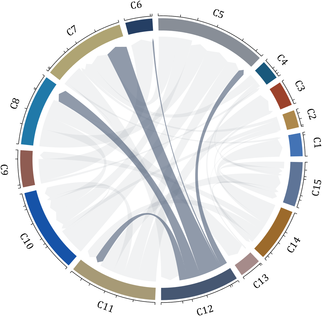
dataMat = rand([15,15]);
dataMat(dataMat > .2) = 0;
CList = [ 75,146,241; 252,180, 65; 224, 64, 10; 5,100,146; 191,191,191;
26, 59,105; 255,227,130; 18,156,221; 202,107, 75; 0, 92,219;
243,210,136; 80, 99,129; 241,185,168; 224,131, 10; 120,147,190]./255;
CListC = [54,69,92]./255;
CList = CList.*.6 + CListC.*.4;
figure('Units','normalized', 'Position',[.02,.05,.6,.85])
BCC = biChordChart(dataMat, 'Arrow','on', 'CData',CList);
BCC = BCC.draw();
% 添加刻度
BCC.tickState('on')
% 修改字体,字号及颜色
BCC.setFont('FontName','Cambria', 'FontSize',17, 'Color',[0,0,0])
% 修改弦颜色(Modify chord color)
for i = 1:size(dataMat, 1)
for j = 1:size(dataMat, 2)
if dataMat(i,j) > 0
BCC.setChordMN(i,j, 'FaceColor',CListC ,'FaceAlpha',.07)
end
end
end
[~, N] = max(sum(dataMat > 0, 2));
for j = 1:size(dataMat, 2)
BCC.setChordMN(N,j, 'FaceColor',CList(N,:) ,'FaceAlpha',.6)
end
You need to download following tools:
- - Chord chart: [chord chart](https://www.mathworks.com/matlabcentral/fileexchange/116550-chord-chart)
- - Directed graph chord chart: [digraph chord chart]:(https://www.mathworks.com/matlabcentral/fileexchange/121043-digraph-chord-chart)
You reached this milestone by providing valuable contribution to the community since you started answering questions in Since September 2011.
You were very active in the first year, and took some break, but you steadily rose ranks in the recent years to achieve this milestone.
You provided 3954 answers and received 1503 votes. You are ranked #25 in the community. Thank you for your contribution to the community and please keep up the good track record!
MATLAB Central Team
In honor of National Pet Day on April 11th, we're excited to announce a fun contest that combines two of our favorite things: our beloved pets and our passion for MATLAB/Simulink! Whether you're a cat enthusiast, a dog lover, or a companion to any other pet, we invite you to join in the fun and showcase your creativity.
How to Participate:
- Take a photo of your pet featuring any element of MATLAB/Simulink.
- Post it in the Fun channel of the Discussions area.
- Include a brief description or story behind the photo - we love to hear about your pets and your creative process!
🏆 Prizes:
We will be selecting 3 winners for this contest, and each winner will receive a MathWorks T-shirt or hat! Winners will be chosen based on creativity, originality, and how well they incorporate the MATLAB/Simulink element into their photo.
📅Important Dates:
Contest ends on April 12th, 2024, at 11:59:59 pm, Eastern Time
We can't wait to see all of your adorable and creative pet photos. Let's celebrate National Pet Day in true MathWorks style. Good luck, and most importantly, have fun!

I'm excited to share some valuable resources that I've found to be incredibly helpful for anyone looking to enhance their MATLAB skills. Whether you're just starting out, studying as a student, or are a seasoned professional, these guides and books offer a wealth of information to aid in your learning journey.
These materials are freely available and can be a great addition to your learning resources. They cover a wide range of topics and are designed to help users at all levels to improve their proficiency in MATLAB.
Happy learning and I hope you find these resources as useful as I have!
I found this link posted on Reddit.
https://workhunty.com/job-blog/where-is-the-best-place-to-be-a-programmer/Matlab/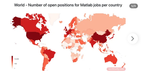
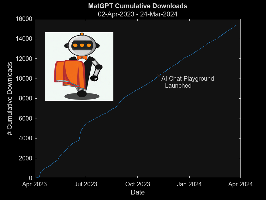
MatGPT was launched on March 22, 2023 and I am amazed at how many times it has been downloaded since then - close to 16,000 downloads in one year. When AI Chat Playground came out on MATLAB Central, I thought surely that people will stop using MatGPT. Boy I was wrong.
In early 2023 I was playing with the new shiny toy called ChatGPT like everyone else but instead of having it tell me jokes or haiku, I wanted to know how I can use it on MATLAB, and I started collecting the prompts that worked. Someone suggested I should turn that into an app, and MatGPT was born with help from other colleagues.
Here is the question - what should I do with it now? Some people suggested I could add other LLMs like Gemini or Claude, but I am more interested in learning how people actually use it.
If you are a MatGPT user, do you mind sharing how you use the app?
Let S be the closed surface composed of the hemisphere 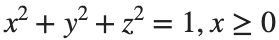 and the base
  Let
Let  be the electric field defined by
 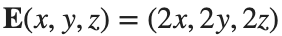 . Find the electric flux through S. (Hint: Divide S into two parts and calculate
  ).
).
% Define the limits of integration for the hemisphere S1
theta_lim = [-pi/2, pi/2];
phi_lim = [0, pi/2];
% Perform the double integration over the spherical surface of the hemisphere S1
% Define the electric flux function for the hemisphere S1
flux_function_S1 = @(theta, phi) 2 * sin(phi);
electric_flux_S1 = integral2(flux_function_S1, theta_lim(1), theta_lim(2), phi_lim(1), phi_lim(2));
% For the base of the hemisphere S2, the electric flux is 0 since the electric
% field has no z-component at the base
electric_flux_S2 = 0;
% Calculate the total electric flux through the closed surface S
total_electric_flux = electric_flux_S1 + electric_flux_S2;
% Display the flux calculations
disp(['Electric flux through the hemisphere S1: ', num2str(electric_flux_S1)]);
disp(['Electric flux through the base of the hemisphere S2: ', num2str(electric_flux_S2)]);
disp(['Total electric flux through the closed surface S: ', num2str(total_electric_flux)]);
% Parameters for the plot
radius = 1; % Radius of the hemisphere
% Create a meshgrid for theta and phi for the plot
[theta, phi] = meshgrid(linspace(theta_lim(1), theta_lim(2), 20), linspace(phi_lim(1), phi_lim(2), 20));
% Calculate Cartesian coordinates for the points on the hemisphere
x = radius * sin(phi) .* cos(theta);
y = radius * sin(phi) .* sin(theta);
z = radius * cos(phi);
% Define the electric field components
Ex = 2 * x;
Ey = 2 * y;
Ez = 2 * z;
% Plot the hemisphere
figure;
surf(x, y, z, 'FaceAlpha', 0.5, 'EdgeColor', 'none');
hold on;
% Plot the electric field vectors
quiver3(x, y, z, Ex, Ey, Ez, 'r');
% Plot the base of the hemisphere
[x_base, y_base] = meshgrid(linspace(-radius, radius, 20), linspace(-radius, radius, 20));
z_base = zeros(size(x_base));
surf(x_base, y_base, z_base, 'FaceColor', 'cyan', 'FaceAlpha', 0.3);
% Additional plot settings
colormap('cool');
axis equal;
grid on;
xlabel('X');
ylabel('Y');
zlabel('Z');
title('Hemisphere and Electric Field');
isempty( [ ] )
10%
isempty( { } )
13%
isempty( '' ) % 2 single quotes
13%
isempty( "" ) % 2 double quotes
24%
c = categorical( [ ] ); isempty(c)
18%
s = struct("a", [ ] ); isempty(s.a)
22%
1324 个投票
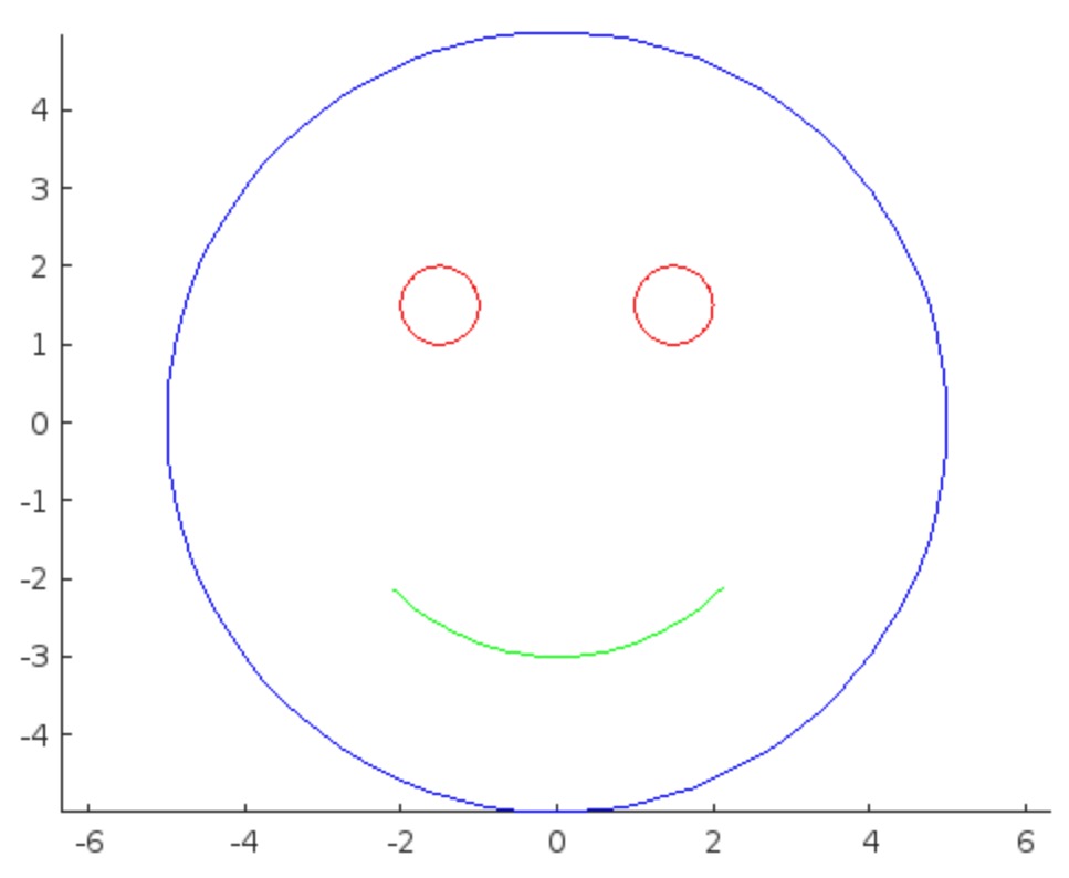
I was in a meeting the other day and a coworker shared a smiley face they created using the AI Chat Playground. The image looked something like this:
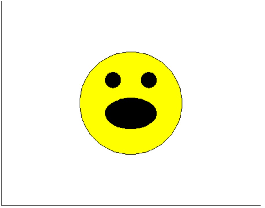
And I suspect the prompt they used was something like this:
"Create a smiley face"
I imagine this output wasn't what my coworker had expected so he was left thinking that this was as good as it gets without manually editing the code, and that the AI Chat Playground couldn't do any better.
I thought I could get a better result using the Playground so I tried a more detailed prompt using a multi-step technique like this:
"Follow these instructions:
- Create code that plots a circle
- Create two smaller circles as eyes within the first circle
- Create an arc that looks like a smile in the lower part of the first circle"
The output of this prompt was better in my opinion.
These queries/prompts are examples of 'zero-shot' prompts, the expectation being a good result with just one query. As opposed to a back-and-forth chat session working towards a desired outcome.
I wonder how many attempts everyone tries before they decide they can't anything more from the AI/LLM. There are times I'll send dozens of chat queries if I feel like I'm getting close to my goal, while other times I'll try just one or two. One thing I always find useful is seeing how others interact with AI models, which is what inspired me to share this.
Does anyone have examples of techniques that work well? I find multi-step instructions often produces good results.
Looking for 10 candidates for a closed beta on new MATLAB live script features.
Do you use live scripts regularly in MATLAB? Do you collaborate with others using live scripts?
MathWorks is looking for 10 candidates for a closed beta on new features for live scripts. Help us develop exciting new features with your feedback.
If you are selected, you will receive an email invitation to sign an NDA
I will post here when the quota is filled

The image was created with DALL-E 3.
Hello, brilliant minds of our engineering community!
We hope this message finds you in the midst of an exciting project or, perhaps, deep in the realms of a challenging problem, because we've got some groundbreaking news that might just make your day a whole lot more interesting.

🎉 Introducing PreAnswer AI - The Future of Community Support! 🎉
Have you ever found yourself pondering over a complex problem, wishing for an answer to magically appear before you even finish formulating the question? Well, wish no more! The MathWorks team, in collaboration with the most imaginative minds from the realms of science fiction, is thrilled to announce the launch of PreAnswer AI, an unprecedented feature set to revolutionize the way we interact within our MATLAB and Simulink community.
What is PreAnswer AI?
PreAnswer AI is our latest AI-driven initiative designed to answer your questions before you even ask them. Yes, you read that right! Through a combination of predictive analytics, machine learning, and a pinch of engineering wizardry, PreAnswer AI anticipates the challenges you're facing and provides you with solutions, insights, and code snippets in real-time.
How Does It Work?
- Presentiment Algorithms: By simply logging into MATLAB Central, our AI begins to analyze your recent coding patterns, activity, and even the intensity of your keyboard strokes to understand your current state of mind.
- Predictive Insights: Using a complex algorithm, affectionately dubbed "The Oracle", PreAnswer AI predicts the questions you're likely to ask and compiles comprehensive answers from our vast database of resources.
- Efficiency and Speed: Imagine the time saved when the answers to your questions are already waiting for you. PreAnswer AI ensures you spend more time innovating and less time searching for solutions.
We are on the cusp of deploying PreAnswer AI in a beta phase and are eager for you to be among the first to experience its benefits. Your feedback will be invaluable as we refine this feature to better suit our community's needs.
---------------------------------------------------------------
Spoiler, it's April 1st if you hadn't noticed. While we might not (yet) have the technology to read minds or predict the future, we do have an incredible community filled with knowledgeable, supportive members ready to tackle any question you throw their way.
Let's continue to collaborate, innovate, and solve complex problems together, proving that while AI can do many things, the power of a united community of brilliant minds is truly unmatched.
Thank you for being such a fantastic part of our community. Here's to many more questions, answers, and shared laughs along the way.
Happy April Fools' Day!
The line integral  , where C is the boundary of the square
  oriented counterclockwise, can be evaluated in two ways:
, where C is the boundary of the square Using the definition of the line integral:
% Initialize the integral sum
integral_sum = 0;
% Segment C1: x = -1, y goes from -1 to 1
y = linspace(-1, 1);
x = -1 * ones(size(y));
dy = diff(y);
integral_sum = integral_sum + sum(-x(1:end-1) .* dy);
% Segment C2: y = 1, x goes from -1 to 1
x = linspace(-1, 1);
y = ones(size(x));
dx = diff(x);
integral_sum = integral_sum + sum(y(1:end-1).^2 .* dx);
% Segment C3: x = 1, y goes from 1 to -1
y = linspace(1, -1);
x = ones(size(y));
dy = diff(y);
integral_sum = integral_sum + sum(-x(1:end-1) .* dy);
% Segment C4: y = -1, x goes from 1 to -1
x = linspace(1, -1);
y = -1 * ones(size(x));
dx = diff(x);
integral_sum = integral_sum + sum(y(1:end-1).^2 .* dx);
disp(['Direct Method Integral: ', num2str(integral_sum)]);
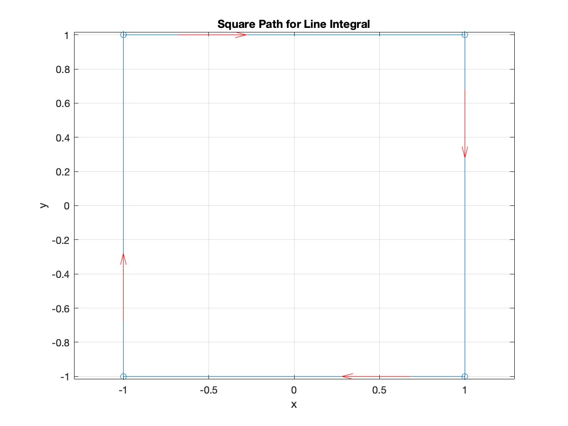
Plotting the square path
% Define the square's vertices
vertices = [-1 -1; -1 1; 1 1; 1 -1; -1 -1];
% Plot the square
figure;
plot(vertices(:,1), vertices(:,2), '-o');
title('Square Path for Line Integral');
xlabel('x');
ylabel('y');
grid on;
axis equal;
% Add arrows to indicate the path direction (counterclockwise)
hold on;
for i = 1:size(vertices,1)-1
% Calculate direction
dx = vertices(i+1,1) - vertices(i,1);
dy = vertices(i+1,2) - vertices(i,2);
% Reduce the length of the arrow for better visibility
scale = 0.2;
dx = scale * dx;
dy = scale * dy;
% Calculate the start point of the arrow
startx = vertices(i,1) + (1 - scale) * dx;
starty = vertices(i,2) + (1 - scale) * dy;
% Plot the arrow
quiver(startx, starty, dx, dy, 'MaxHeadSize', 0.5, 'Color', 'r', 'AutoScale', 'off');
end
hold off;
Apply Green's Theorem for the line integral
% Define the partial derivatives of P and Q
f = @(x, y) -1 - 2*y; % derivative of -x with respect to x is -1, and derivative of y^2 with respect to y is 2y
% Compute the double integral over the square [-1,1]x[-1,1]
integral_value = integral2(f, -1, 1, 1, -1);
disp(['Green''s Theorem Integral: ', num2str(integral_value)]);
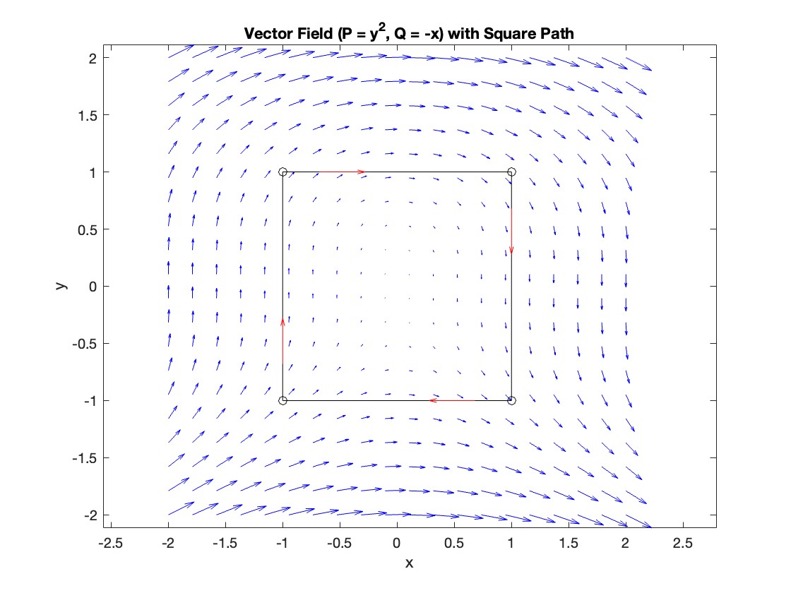
Plotting the vector field related to Green’s theorem
% Define the grid for the vector field
[x, y] = meshgrid(linspace(-2, 2, 20), linspace(-2 ,2, 20));
% Define the vector field components
P = y.^2; % y^2 component
Q = -x; % -x component
% Plot the vector field
figure;
quiver(x, y, P, Q, 'b');
hold on; % Hold on to plot the square on the same figure
% Define the square's vertices
vertices = [-1 -1; -1 1; 1 1; 1 -1; -1 -1];
% Plot the square path
plot(vertices(:,1), vertices(:,2), '-o', 'Color', 'k'); % 'k' for black color
title('Vector Field (P = y^2, Q = -x) with Square Path');
xlabel('x');
ylabel('y');
axis equal;
% Add arrows to indicate the path direction (counterclockwise)
for i = 1:size(vertices,1)-1
% Calculate direction
dx = vertices(i+1,1) - vertices(i,1);
dy = vertices(i+1,2) - vertices(i,2);
% Reduce the length of the arrow for better visibility
scale = 0.2;
dx = scale * dx;
dy = scale * dy;
% Calculate the start point of the arrow
startx = vertices(i,1) + (1 - scale) * dx;
starty = vertices(i,2) + (1 - scale) * dy;
% Plot the arrow
quiver(startx, starty, dx, dy, 'MaxHeadSize', 0.5, 'Color', 'r', 'AutoScale', 'off');
end
hold off;
您也可以从以下列表中选择网站:
美洲
- América Latina (Español)
- Canada (English)
- United States (English)
欧洲
- Belgium (English)
- Denmark (English)
- Deutschland (Deutsch)
- España (Español)
- Finland (English)
- France (Français)
- Ireland (English)
- Italia (Italiano)
- Luxembourg (English)
- Netherlands (English)
- Norway (English)
- Österreich (Deutsch)
- Portugal (English)
- Sweden (English)
- Switzerland
- United Kingdom(English)
亚太
- Australia (English)
- India (English)
- New Zealand (English)
- 中国
- 日本Japanese (日本語)
- 한국Korean (한국어)