How to Perform Curve Fitting Using the Curve Fitting App in MATLAB
Learn how to perform curve fitting in MATLAB® using the Curve Fitting app and fit noisy data using smoothing spline. You can use the Curve Fitting app interactively to try a variety of fitting algorithms, assess the fit numerically, and generate code from the app.
Published: 14 Feb 2021
In this video, we will show you how to perform curve fitting in MATLAB for math modeling applications. Curve fitting is the process of constructing a curve or mathematical function that has the best fit to a series of data points. In a way, summarize the relationship among these variables.
In this video, we will see interactive curve fitting using the curve fitting app. Before you can fit data, you need to load the data variables into the MATLAB workspace. For this example, we load some basic US population data that is available in MATLAB at census.mat.
We can see the workspace has the variables cdate and pop. Pop is the population that corresponds to the years in cdate. We now create a basic plot of the two variables.
We can open the curve fitting tool by clicking on the Apps tab and selecting Curve Fitting or by typing CF Tool and then running the section. To load cdate and pop into the curve fitting tool, select them as x data and y data, respectively.
The default effort is a linear polynomial fit of degree 1. The curve fitting app allows you to explore many different functions, including Exponential, Fourier, and Power to name a few. And you can evaluate their goodness of fit.
For example, change the fit to a second-degree polynomial by selecting 2 from the degree list and observe how much the fit improves both visually and in the Goodness of Fit measures like sum of squared arrow. The Curve Fitting toolbox has functions that allow you to construct splines for fitting to and smoothing data.
If your data is noisy, you might want to fit it using a smoothing spline. Splines are smooth piecewise polynomials that can be used to represent functions over large intervals, but it would be impractical to use a single approximating polynomial.
Let us load carbon-12 alpha into the workspace. In the curve fitting app, load Angle and Counts. Select them as x and y data, respectively. Select the smoothing spline fit type.
The toolbox attempts to select a default value appropriate for your data. The default smoothing parameter produces the smoothest curve. To make a smoother fit further from the data, click the Smoother button repeatedly until the plot shows the smoothness you want.
Similarly, to make a ruffle closer to the data, click the Ruffle button until you are satisfied with the plot. Click Default to return to the initial value. The app keeps track of the various fits you tried. Select File, click Generate Code to create a MATLAB function to recreate all fits and plots in your interactive session.
In conclusion, we discussed how to perform curve fitting in MATLAB using the curve fitting app and fitting noisy data using smoothing spline. The curve fitting app helps you try a variety of algorithms interactively, assess the fit numerically and visually, and generate code from the app. If you want to learn more about the curve fitting toolbox and its functionalities that we used in this video, feel free to go through the links in the description.


