Parachute Simulation Study with Monte Carlo Analysis
This example shows the simulation of a package with a parachute being dropped from an airplane. The parachute opens out of the package and induces a drag force, slowing the descent. The example uses Monte Carlo analysis to perform the sensitivity study of the parachute simulation with uncertainty in wind disturbance, airdrop altitude of the package from the aircraft, and opening altitude of the parachute.
Simulink Model Description
To understand the parachute simulation architecture, open the Simulink™ model.
open_system('ParachuteSim.slx');The top model consists of two subsystems:
Environment defines the environment in which the parachute operates. It consists of the following blocks:
Flat Earth to LLA block converts Earth position to latitude, longitude, and altitude. The initial heading angle and the initial latitude and longitude of the package drop are specified as parameters in the block. The variable headingInitial corresponds to the initial heading angle in degrees. The variables latInitial and longInitial correspond to the geodetic latitude and longitude in degrees.
headingInitial =45; latInitial =
43.5319; longInitial =
1.2438;
COESA Atmosphere Model calculates the density value corresponding to the altitude.
WGS84 Gravity Model computes the Earth gravity at a specific latitude, longitude, and altitude.
A realistic wind environment is created using the combination of Wind Shear Model to calculate the mean wind speed, Dryden Wind Turbulence Model (Continuous) to add wind turbulence, and Discrete Wind Gust Model to generate gust wind.
Parachute System Model uses the 6DOF (Euler Angles) block to simulate the parachute model based on the initial conditions, weight, and drag force. When a package containing the parachute is dropped from an aircraft, two forces act on it, the weight of the package and the aerodynamic drag. The aerodynamic drag force of the package is negligible before the parachute opens, resulting in a projectile motion of the package. Once the parachute opens, the aerodynamic drag on the parachute slows the descent. The default values of the parachute are based on the EPC (Ensemble de Parachutage du Combattant), one of the French parachutes manufactured by IrvinGQ (formerly Airborne Systems).
As the aerodynamic drag and the weight of the parachute are opposing forces, the net vertical force is given by the difference between the weight and the drag force , where:
mass represents the mass of the parachute in kg
g is the acceleration due to gravity approximated to 9.81
rho is the density of air approximated to 1.229
velocity corresponds to the velocity of parachute in
is the drag coefficient
area represents the area of the parachute in
During the descent, a point is quickly reached when the net force on the parachute is zero and the drag equals weight. This relation is used to compute the drag coefficient of the parachute, as follows:
area =115; mass =
165; velocity =
6; g = 9.81; rho = 1.229; Cd = 2*mass*g/(rho*(velocity^2)*area);
The gravity and density values corresponding to the altitude and wind velocity computed in the Environment subsystem are used with the drag coefficient, opening altitude, and mass of the parachute to obtain the net force acting on the parachute. The opening altitude, denoted by the variable hOpening, corresponds to the altitude (in meters) at which the parachute is deployed from the package. Observe that the opening altitude should be less than the airdrop altitude from an aircraft. The variable packageMass corresponds to the mass of the package with the parachute in kg. By default, the opening altitude and the package mass are set to 500 m and 130 kg, respectively.
hOpening =500; packageMass =
130;
The net moments on the parachute are assumed zero. The net forces and moments are subsequently fed to the 6DOF (Euler Angles) block to simulate the parachute model based on the specified initial conditions in the block. The initial position in the inertial axis is specified below. The variable ZeInitial corresponds to the airdrop altitude (in meters) of the package from the aircraft. By default, the airdrop altitude of the package is set to 2000 m.
XeInitial =0; YeInitial =
0; ZeInitial =
2000;
The initial velocity of the package along the x-axis corresponds to the velocity of the aircraft when the package is dropped, and is given a default value of 235 km/h. The initial velocities of the package along y and z-axes are considered zero (in km/h). The initial Euler angle and Euler rates are considered zero. The initial velocities in the three body axes are converted to m/s using the convvel function as shown below:
UInitialKMPH =235; UInitialMPS = convvel(UInitialKMPH,'km/h','m/s'); VInitialKMPH =
0; VInitialMPS = convvel(VInitialKMPH,'km/h','m/s'); WInitialKMPH =
0; WInitialMPS = convvel(WInitialKMPH,'km/h','m/s');
Parachute Simulation
By default, the wind disturbance is introduced in the parachute simulation. The parameter Gust start time in Discrete Wind Gust Model corresponds to the time the gust begins. As the time taken for the parachute to reach the ground is around 100 seconds, the variable windSeed that corresponds to the Gust start time parameter is taken as a random integer within a range of 1 to 100 using the randi function. To simulate the parachute model without wind disturbance, set the windDisturbance variable to false. This switching is carried out in the Simulink model using a Variant Subsystem with windDisturbance as the variant choice variable.
windDisturbance =true; if windDisturbance == true windSeed = randi(100,1); end
After initializing and setting up all the parameters of the parachute simulation model, the sim function simulates it until the parachute touches the ground. The results are stored in the variable SimResults as a Simulink.SimulationOutput object.
simResults = sim('ParachuteSim.slx');The simulation results characterize the response of the parachute. An overview is given by the state of the parachute at the touchdown, as follows.
The time taken for the parachute to hit the ground in seconds:
TFinal = simResults.tout(end)
TFinal =
107.9866
The position along the x-axis where the parachute hits the ground in meters:
XeFinal = simResults.yout{1}.Values.Data(end,1) XeFinal = 1.0795e+03
The position along the y-axis where the parachute hits the ground in meters:
YeFinal = simResults.yout{1}.Values.Data(end,2) YeFinal = -255.7525
The velocity along the x-axis with which the parachute hits the ground in m/s:
UeFinal = simResults.yout{2}.Values.Data(end,1) UeFinal = -1.9809
The velocity along the y-axis with which the parachute hits the ground in m/s:
VeFinal = simResults.yout{2}.Values.Data(end,2) VeFinal = -3.0081
The velocity along the z-axis with which the parachute hits the ground in m/s:
WeFinal = simResults.yout{2}.Values.Data(end,3) WeFinal = -5.3138
The variables YeFinal and VeFinal depend on the wind disturbance. If an ideal scenario with no wind condition is considered, then these variables are zero. This assumption results in only longitudinal motion of the parachute, represented in 2D with x and z coordinates. However, in a realistic environment, the package exhibits both lateral and longitudinal motion, which is plotted below in 3D. From the plot, observe that the package exhibits a projectile motion until the parachute opens and induces an aerodynamic drag. This drag considerably slows down the descent.
figure;
plot3(simResults.yout{1}.Values.Data(:,1),simResults.yout{1}.Values.Data(:,2),...
      simResults.yout{1}.Values.Data(:,3));
zlim([0 max(simResults.yout{1}.Values.Data(:,3))]);
grid on;
xlabel('Xe (m)');
ylabel('Ye (m)');
zlabel('Ze (m)');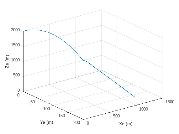
The planar satellite view of the parachute simulation is depicted below. The flat2lla function estimates latitude, longitude, and altitude from the Earth position coordinates. The geoplot function plots the resulting geographic coordinates. The geobasemap function changes the basemap to satellite.
figure;
llaPosition = flat2lla([simResults.yout{1}.Values.Data(:,1) ...
                        simResults.yout{1}.Values.Data(:,2) ...
                     -1*simResults.yout{1}.Values.Data(:,3)],...
                     [latInitial, longInitial], headingInitial,0);
geoplot(llaPosition(:,1), llaPosition(:,2),'r','LineWidth',2)
geolimits([min(llaPosition(:,1))-0.01 max(llaPosition(:,1))+0.01],...
          [min(llaPosition(:,2))-0.01 max(llaPosition(:,2))+0.01])
geobasemap satellite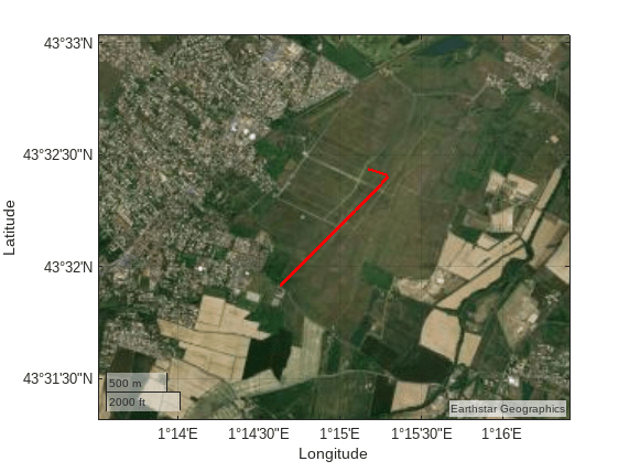
Monte Carlo Analysis Using Parallel Simulation
The Monte Carlo simulations assess the response of the parachute under uncertain conditions. The variable numSim provides the number of simulations in the Monte Carlo analysis. In the parachute simulation, the uncertainty in wind disturbance, airdrop altitude of the package, and the opening altitude of the parachute are considered. The randomness in wind disturbance is accommodated by varying the start time of the gust in the Discrete Wind Gust Model block within the range of 1 to 100.
numSim             = 100;
windDisturbance    = true;
gustStartTime      = randi(100,[1 numSim]);
The uncertainty in the airdrop altitude of the package and the opening altitude of the parachute is assumed to follow a normal distribution curve with the mean set at the initial conditions of ZeInitial and hOpening, respectively. The standard deviations of the airdrop altitude and the opening altitude are specified below:
ZeDeviation =5; hOpeningDeviation =
5;
The random values of the airdrop altitude and the opening altitude are then drawn from a normal distribution with the specified mean and standard deviation using the randn function.
airdropAltitude = ZeDeviation.*randn(numSim,1) + ZeInitial;
openingAltitude = hOpeningDeviation.*randn(numSim,1) + hOpening;
The Monte Carlo analysis requires simulating the parachute system multiple times, so this example uses the parsim function. The Simulink.SimulationInput object specifies the varying inputs of the simulations. The parsim function is configured to run simulations using fast restart, to monitor progress using Simulation Manager, to track the progress of simulations, and to transfer the variables in the base workspace to the parallel workers using Parallel Computing Toolbox™.
in(1:numSim) = Simulink.SimulationInput('ParachuteSim');
for simNumber = 1:1:numSim
    in(simNumber) = in(simNumber).setVariable('hOpening',openingAltitude(simNumber));
    in(simNumber) = in(simNumber).setVariable('Ze',airdropAltitude(simNumber));
    in(simNumber) = in(simNumber).setVariable('windSeed',gustStartTime(simNumber));
end
simResults = parsim(in, 'UseFastRestart','on','ShowSimulationManager', 'on',...
                    'ShowProgress','on','TransferBaseWorkspaceVariables','on');
[19-Dec-2024 17:47:06] Checking for availability of parallel pool...
Starting parallel pool (parpool) using the 'Processes' profile ...
19-Dec-2024 17:48:29: Job Queued. Waiting for parallel pool job with ID 1 to start ...
Connected to parallel pool with 6 workers.
[19-Dec-2024 17:49:10] Starting Simulink on parallel workers...
[19-Dec-2024 17:50:09] Configuring simulation cache folder on parallel workers...
[19-Dec-2024 17:50:10] Transferring base workspace variables used in the model to parallel workers...
[19-Dec-2024 17:50:10] Total size of base workspace variables to send to parallel workers is 338.21 KB.
[19-Dec-2024 17:50:11] Loading model on parallel workers...
[19-Dec-2024 17:50:44] Running simulations...
[19-Dec-2024 17:52:16] Cleaning up parallel workers...
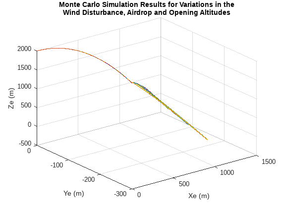
The results of the multiple simulations are plotted below. From the plot, it is seen that the input uncertainties result in a small deviation of the landing site of the parachute.
figure;
for simNumber = 1:1:numSim
    plot3(simResults(1,simNumber).yout{1}.Values.Data(:,1),...
          simResults(1,simNumber).yout{1}.Values.Data(:,2),...
          simResults(1,simNumber).yout{1}.Values.Data(:,3));
    hold on;
end
grid on;
title(["Monte Carlo Simulation Results for Variations in the";...
       "Wind Disturbance, Airdrop and Opening Altitudes"]);
xlabel('Xe (m)');
ylabel('Ye (m)');
zlabel('Ze (m)');
The simulation results are also represented as a geoplot in the satellite view.
figure;
gx = geoaxes;
for simNumber = 1:1:numSim
    llaPosition = flat2lla([simResults(1,simNumber).yout{1}.Values.Data(:,1) ...
                            simResults(1,simNumber).yout{1}.Values.Data(:,2) ...
                           -1*simResults(1,simNumber).yout{1}.Values.Data(:,3)],...
                           [latInitial, longInitial], headingInitial,0);
    geoplot(gx,llaPosition(:,1), llaPosition(:,2),'LineWidth',2)
    geolimits(gx,[min(llaPosition(:,1,:))-0.01 max(llaPosition(:,1,:))+0.01],...
                 [min(llaPosition(:,2,:))-0.01 max(llaPosition(:,2,:))+0.01])
    geobasemap(gx,"satellite")
    hold on
end
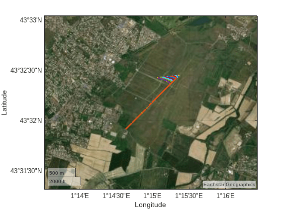
The plot is zoomed in to reflect the differences in the landing sites corresponding to each of the parachute simulations.
figure;
gx = geoaxes;
for simNumber = 1:1:numSim
    llaPosition = flat2lla([simResults(1,simNumber).yout{1}.Values.Data(:,1) ...
                            simResults(1,simNumber).yout{1}.Values.Data(:,2) ...
                         -1*simResults(1,simNumber).yout{1}.Values.Data(:,3)],...
                           [latInitial, longInitial], headingInitial,0);
    geoplot(gx,llaPosition(:,1), llaPosition(:,2),'LineWidth',2)
    geolimits(gx,[43.5375 43.5420],[1.2495 1.2570])
    geobasemap(gx,"satellite")
    hold on
end

The example demonstrates Monte Carlo analysis for parachute simulation with variations in the wind disturbance, airdrop and opening altitudes. Observe the simulation results of Monte Carlo analysis by varying the start time of the wind gust and standard deviations of the airdrop and opening altitudes.
Delete Current Pool
Use the parallel pool object to delete the current pool of parallel workers created by parsim.
delete(gcp('nocreate'));Parallel pool using the 'Processes' profile is shutting down.