Analyze State-Space Model for Linear Control and Static Stability Analysis
This example shows how to convert a fixed-wing aircraft to a linear time invariant (LTI) state-space model for linear analysis.
This example describes:
Importing and filling data from a DATCOM file.
Constructing a fixed-wing aircraft from DATCOM data.
Calculating static stability of the fixed-wing aircraft.
Linearizing the fixed-wing aircraft around an initial state.
Validating the static stability analysis with a dynamic response.
Isolating the elevator-to-pitch transfer function and designing a feedback controller for the elevator.
Defining the Fixed-Wing Aircraft and State
This example uses a DATCOM file created for the Sky Hogg aircraft.
First, import the DATCOM output file using datcomimport.
allData = datcomimport('astSkyHoggDatcom.out', false, 0);
skyHoggData = allData{1}
skyHoggData = struct with fields:
case: 'SKYHOGG BODY-WING-HORIZONTAL TAIL-VERTICAL TAIL CONFIG'
mach: [0.1000 0.2000 0.3000 0.3500]
alt: [1000 3000 5000 7000 9000 11000 13000 15000]
alpha: [-16 -12 -8 -4 -2 0 2 4 8 12]
nmach: 4
nalt: 8
nalpha: 10
rnnub: []
hypers: 0
loop: 2
sref: 225.8000
cbar: 5.7500
blref: 41.1500
dim: 'ft'
deriv: 'deg'
stmach: 0.6000
tsmach: 1.4000
save: 0
stype: []
trim: 0
damp: 1
build: 1
part: 0
highsym: 1
highasy: 0
highcon: 0
tjet: 0
hypeff: 0
lb: 0
pwr: 0
grnd: 0
wsspn: 18.7000
hsspn: 5.7000
ndelta: 5
delta: [-20 -10 0 10 20]
deltal: []
deltar: []
ngh: 0
grndht: []
config: [1×1 struct]
version: 1976
cd: [10×4×8 double]
cl: [10×4×8 double]
cm: [10×4×8 double]
cn: [10×4×8 double]
ca: [10×4×8 double]
xcp: [10×4×8 double]
cma: [10×4×8 double]
cyb: [10×4×8 double]
cnb: [10×4×8 double]
clb: [10×4×8 double]
cla: [10×4×8 double]
qqinf: [10×4×8 double]
eps: [10×4×8 double]
depsdalp: [10×4×8 double]
clq: [10×4×8 double]
cmq: [10×4×8 double]
clad: [10×4×8 double]
cmad: [10×4×8 double]
clp: [10×4×8 double]
cyp: [10×4×8 double]
cnp: [10×4×8 double]
cnr: [10×4×8 double]
clr: [10×4×8 double]
dcl_sym: [5×4×8 double]
dcm_sym: [5×4×8 double]
dclmax_sym: [5×4×8 double]
dcdmin_sym: [5×4×8 double]
clad_sym: [5×4×8 double]
cha_sym: [5×4×8 double]
chd_sym: [5×4×8 double]
dcdi_sym: [10×5×4×8 double]
Next, prepare the DATCOM lookup tables.
DATCOM lookup tables might have missing values due to the tables only filling one value for the whole column.
This missing data is represented in the lookup tables as the value 99999 and can be filled using the "previous" method of fillmissing.
In this example, , , , and have missing data.
skyHoggData.cyb = fillmissing(skyHoggData.cyb, "previous", "MissingLocations", skyHoggData.cyb == 99999);
skyHoggData.cnb = fillmissing(skyHoggData.cnb, "previous", "MissingLocations", skyHoggData.cnb == 99999);
skyHoggData.clq = fillmissing(skyHoggData.clq, "previous", "MissingLocations", skyHoggData.clq == 99999);
skyHoggData.cmq = fillmissing(skyHoggData.cmq, "previous", "MissingLocations", skyHoggData.cmq == 99999);
With the missing data filled, the fixed-wing aircraft can be constructed.
First, the fixed-wing aircraft is prepared with the desired aircraft name.
Optionally, the aircraft name can be extracted from the "case" field on the DATCOM struct by passing an empty fixed-wing object.
skyHogg = Aero.FixedWing();
skyHogg.Properties.Name = "Sky_Hogg";
skyHogg.DegreesOfFreedom = "3DOF";
[skyHogg, cruiseState] = datcomToFixedWing(skyHogg, skyHoggData);
The datcomToFixedWing will convert all compatible data from the datcom struct into the fixed-wing object and its state. However, the returned state still needs processing to get the desired initial conditions of the aircraft.
In this example, the environment, mass, inertia, airspeed, and center of pressure need adjusting.
h = 2000;
cruiseState.AltitudeMSL = h;
cruiseState.Environment = aircraftEnvironment(skyHogg,"ISA",h);

cruiseState.Airspeed = 169.42;
cruiseState.Mass = 1299.214;
cruiseState.Inertia.Variables = [5787.969 0 117.64;0 6928.93 0;-117.64 0 11578.329];
cruiseState.CenterOfPressure = [0.183, 0, 0];
Calculating Static Stability
Performing a static stability analysis helps determine the dynamic stability of the system without calculating a dynamic system response.
stability = staticStability(skyHogg, cruiseState)
stability=6×8 table
             U            V           W         Alpha        Beta           P           Q            R
          ________    _________    ________    ________    _________    _________    ________    _________

    FX    "Stable"    ""           ""          ""          ""           ""           ""          ""
    FY    ""          "Neutral"    ""          ""          ""           ""           ""          ""
    FZ    ""          ""           "Stable"    ""          ""           ""           ""          ""
    L     ""          ""           ""          ""          "Neutral"    "Neutral"    ""          ""
    M     "Stable"    ""           ""          "Stable"    ""           ""           "Stable"    ""
    N     ""          ""           ""          ""          "Neutral"    ""           ""          "Neutral"
With statically stable forces and moments, with perturbations to forward and vertical speeds, and perturbations to angle of attack, the dynamic stability of the system tends towards an oscillating steady-state when perturbing the forward and vertical speeds.
To verify this behavior, use the Control System Toolbox™.
Linearizing the Fixed-Wing Aircraft
To use the tools within the Control System Toolbox, linearize the aircraft around a state.
This is done by using the linearize method with the same cruise state as before.
linSys = linearize(skyHogg, cruiseState)
linSys =

  A =
                  XN          XD           U           W           Q       Theta
   XN              0           0           1  -2.842e-09           0  -2.586e-07
   XD              0           0           0           1           0      -2.957
   U               0   1.319e-06   -0.001714   -0.000759           0     -0.5617
   W               0           0   -0.002705     -0.3319        2.95  -4.903e-08
   Q               0           0     0.03443       -1.19     -0.4252   8.882e-11
   Theta           0           0           0           0           1           0

  B =
               Delta
   XN              0
   XD              0
   U      -0.0004314
   W        -0.02084
   Q          -2.239
   Theta           0

  C =
                  XN          XD           U           W           Q       Theta
   XN              1           0           0           0           0           0
   XD              0           1           0           0           0           0
   U               0           0           1  -2.842e-09           0           0
   W               0           0           0           1           0           0
   Q               0           0           0           0           1           0
   Theta           0           0           0           0           0           1

  D =
          Delta
   XN         0
   XD         0
   U          0
   W          0
   Q          0
   Theta      0

Continuous-time state-space model.
Model Properties
Validating Static Stability with Dynamic Response
With the linear state-space model constructed, you can plot the dynamic behavior of the system.
To verify the static stability results with the dynamic behavior of the system, plot the states space model against the initial conditions.
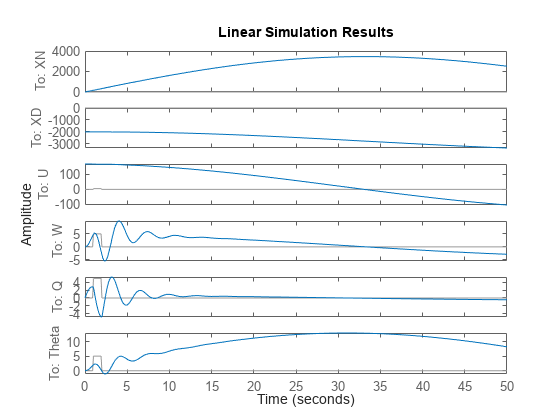
To induce a perturbation in the system, a 5 degree step for 1 second is added to the elevator signal.
x0 = getState(cruiseState, linSys.OutputName);
t = linspace(0, 50, 500);
u = zeros(size(t));
u(t > 1 & t < 2) = 5;
lsim(linSys,u,t,x0)
As expected from the static stability analysis, the airspeed and pitch-rate is stable when responding to a small perturbation in the elevator.
Isolating the Elevator-Pitch Response
In addition to the static stability verification, isolating the control surfaces to their intended dynamic response can help design controllers specific to the individual surfaces.
In this case, there is only a single control surface, the elevator.
The elevator controls the pitch response of the aircraft. To show a pitch response, isolate the elevator input to the pitch angle to elevator transfer function.
linSysElevatorTF = tf(linSys(6,1))
linSysElevatorTF =

  From input "Delta" to output "Theta":
           -2.239 s^3 - 0.7221 s^2 - 0.001232 s - 8.935e-09
  -------------------------------------------------------------------
  s^5 + 0.7587 s^4 + 3.652 s^3 + 0.02567 s^2 + 0.008226 s + 5.711e-08

Continuous-time transfer function.
Model Properties
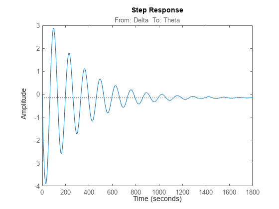
step(linSysElevatorTF)

As can be seen by the step plot, the pitch response to elevator input has an undesirable oscillatory nature and large steady-state error.
By adding a PID feedback controller to the elevator input, a much more desirable pitch response can be achieved.
C = pidtune(linSysElevatorTF, "PID")C =
1
Ki * ---
s
with Ki = -0.00153
Continuous-time I-only controller.
Model Properties
elevatorFeedback = feedback(linSysElevatorTF * C, 1)
elevatorFeedback =

  From input to output "Theta":
                 0.003417 s^3 + 0.001102 s^2 + 1.881e-06 s + 1.364e-11
  -----------------------------------------------------------------------------------
  s^6 + 0.7587 s^5 + 3.652 s^4 + 0.02909 s^3 + 0.009328 s^2 + 1.938e-06 s + 1.364e-11

Continuous-time transfer function.
Model Properties
step(elevatorFeedback)

