Main Content

propagationData

Create RF propagation data from measurements

Since R2020a

Description

Use the propagationData object to import and visualize geolocated propagation data. The measurement data can be path loss data, signal strength measurements, signal-to-noise-ratio (SNR) data, or cellular information.

Creation

Description

pd = propagationData(filename) creates a propagation data object by reading data from a file specified by filename.

pd = propagationData(table) creates a propagation data container object from the specified table.

example

pd = propagationData(latitude,longitude,varname,varvalue) creates a propagation data container object using latitude and longitude coordinates with data specified using varname and varvalue.

example

pd = propagationData(___,Name,Value) sets properties using one or more name-value pairs. Enclose each property name in quotes.

Input Arguments

expand all

Name of the file containing propagation data, specified as a character vector or a string scalar. The file must be in the current directory, in a directory on the MATLAB path, or be specified using a full or relative path. The file must be compatible with the readtable function. Call the readtable function if customized parameters are required to import the file and then pass the table to the propagationData object.

Propagation data in the file must have one variable corresponding to the latitude values, one variable corresponding to longitude values, and at least one variable containing numeric data.

Data Types: string | char

Table containing propagation data. The table must have one variable corresponding to latitude values, one variable corresponding to longitude values, and at least one variable containing numeric data.

Data Types: table

Latitude coordinate values, specified as a vector in decimal degrees with reference to Earth's ellipsoid model WGS-84. The latitude coordinates must be in the range [-90 90].

Data Types: double

Longitude coordinate values, specified as a vector in decimal degrees with reference to earth's ellipsoid. model WGS-84.

Data Types: double

Variable name, specified as a character vector or a string scalar. This variable name must correspond to a variable with numeric data (other than latitude or longitude). The variable name and the corresponding values are stored as a variable in the table stored in Data.

Data Types: string | char

Variable values, specified as a numeric vector. The numeric vectors must be the same size as latitude and longitude. The variable name and the corresponding values are stored as a variable in the table stored in Data.

Data Types: double

Output Arguments

expand all

Propagation data, returned as a propagationData object.

Properties

expand all

Propagation data name, specified as a character vector or string scalar.

Example: 'Name','propdata'

Example: pd.Name = 'propdata'

Data Types: char | string

This property is read-only.

Propagation data table, specified as a table that contains a variable corresponding to latitude coordinates, a variable corresponding to longitude coordinates, and one or more variables corresponding to associated propagation data.

Data Types: table

Name of the data variable to plot, specified as a character vector or string scalar corresponding to a variable name in the Data table used to create propagation data container object. The variable name must correspond to a variable with numeric data and cannot correspond to the latitude or longitude variables. The default value for this property is the name of the first numeric data variable name in the Data table that is not a latitude or longitude variable.

Data Types: char | string

Object Functions

plotDisplay RF propagation data in Site Viewer
contourDisplay contour map of RF propagation data in Site Viewer
locationCoordinates of RF propagation data
getDataVariableGet data variable values
interpInterpolate RF propagation data

Examples

collapse all

Launch Site Viewer with basemaps and building files for Manhattan. For more information about the OpenStreetMap® file, see [1].

viewer = siteviewer("Basemap","streets_dark",...
        "Buildings","manhattan.osm");

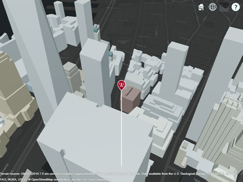
Show a transmitter site on a building.

tx = txsite("Latitude",40.7107,...
        "Longitude",-74.0114,...
        "AntennaHeight",80);
show(tx)

Create receiver sites along nearby streets.

latitude = [linspace(40.7088, 40.71416, 50), ...
        linspace(40.71416, 40.715505, 25), ...
        linspace(40.715505, 40.7133, 25), ...
        linspace(40.7133, 40.7143, 25)]';
longitude = [linspace(-74.0108, -74.00627, 50), ...
        linspace(-74.00627 ,-74.0092, 25), ...
        linspace(-74.0092, -74.0110, 25), ...
        linspace(-74.0110, -74.0132, 25)]';
rxs = rxsite("Latitude", latitude, "Longitude", longitude);

Compute signal strength at each receiver location.

signalStrength = sigstrength(rxs, tx)';

Create a propagationData object to hold computed signal strength data.

tbl = table(latitude, longitude, signalStrength);
pd = propagationData(tbl);

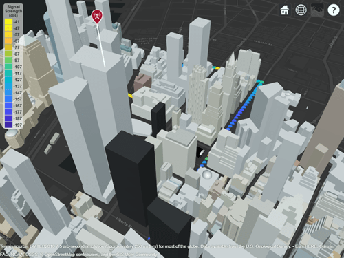
Plot the signal strength data on a map as colored points.

legendTitle = "Signal" + newline + "Strength" + newline + "(dB)";
plot(pd, "LegendTitle", legendTitle, "Colormap", parula);

Appendix

[1] The OpenStreetMap file is downloaded from https://www.openstreetmap.org, which provides access to crowd-sourced map data all over the world. The data is licensed under the Open Data Commons Open Database License (ODbL), https://opendatacommons.org/licenses/odbl/.

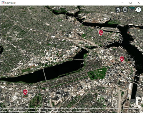
Define names and locations of sites around Boston.

names = ["Fenway Park","Faneuil Hall","Bunker Hill Monument"];
lats = [42.3467,42.3598,42.3763];
lons = [-71.0972,-71.0545,-71.0611];

Create an array of transmitter sites.

txs = txsite("Name",names,...
       "Latitude",lats,...
       "Longitude",lons, ...
       "TransmitterFrequency",2.5e9);
show(txs)

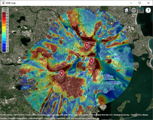
Create a signal-to-interference-plus-noise-ratio (SINR) map, where signal source for each location is selected as the transmitter site with the strongest signal.

sv1 = siteviewer("Name","SINR map");
sinr(txs,"MaxRange",5000)

Return SINR propagation data.

pd = sinr(txs,"MaxRange",5000);
[sinrDb,lats,lons] = getDataVariable(pd,"SINR"); 

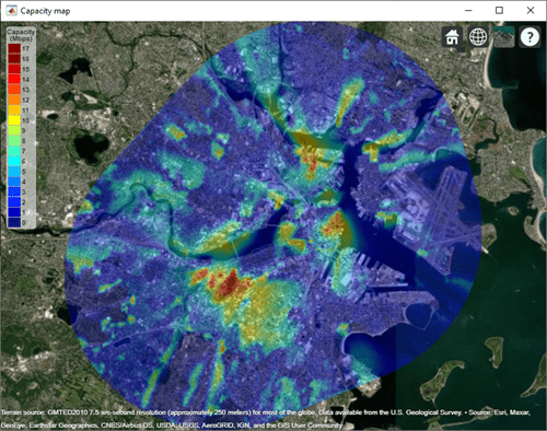
Compute capacity using the Shannon-Hartley theorem.

bw = 1e6; % Bandwidth is 1 MHz
sinrRatio = 10.^(sinrDb./10); % Convert from dB to power ratio
capacity = bw*log2(1+sinrRatio)/1e6; % Unit: Mbps

Create new propagation data for the capacity map and display the contour plot.

pdCapacity = propagationData(lats,lons,"Capacity",capacity);
sv2 = siteviewer("Name","Capacity map");
legendTitle = "Capacity" + newline + "(Mbps)";
contour(pdCapacity,"LegendTitle",legendTitle);

Version History

Introduced in R2020a