Frequency Response and Surface Plot Analysis
This example shows how to perform frequency response analysis and evaluate surface plot characteristics of an AI-model-based horn antenna. Using AI-based modeling, this example generates these surface plots in just a few seconds, enabling rapid exploration of the design space. In this example, you vary the tunable parameters of the AI-based antenna by ±15%, and sweep the operating frequency over a ±30% range around the design frequency.
To evaluate the horn antenna's performance across the frequency band, carry out the beamwidth and peak gain analyses from **–**30% to +30% around the design frequency. This frequency sweep helps illustrate the typical antenna design tradeoff: as gain increases, beamwidth generally decreases, and vice versa. This approach allows you to visually identify optimal parameter combinations and understand key performance tradeoff without the need for manual tuning.
Create AI Model Based Horn Antenna
Create an AI-based horn antenna using the design function by setting the ForAI argument to true.
f = 10e9;
ant = horn;
antAI = design(ant,f,ForAI=true);
Analyze Frequency Response
Define the frequency sweep.
freqall = linspace(0.7*f,1.3*f,101);
nf = numel(freqall);
bwall = zeros(1,nf); % Beamwidth at all frequency points
pgall = zeros(1,nf); % Peak gain at all frequency points
Perform beamwidth and peak radiation analyses. Measure the time taken to calculate the beamwidth and peak gain at 101 frequency points.
tic
for i = 1: numel(freqall)
    [bw, ang, ~] = beamwidth(antAI,freqall(i));
    bwall(i) = bw(1);
    [pgall(i), ~,~] = peakRadiation(antAI,freqall(i));
end
tfreq = toc
tfreq =
0.6171
Plot frequency versus beamwidth and frequency versus peak gain.
figure
plot(freqall,bwall)
ylabel("beamwidth");
yyaxis right;

plot(freqall,pgall);
ylabel("peak gain");
xlabel("frequency");
title("beamwidth vs peak gain")
legend({"beamwidth","peak gain"})
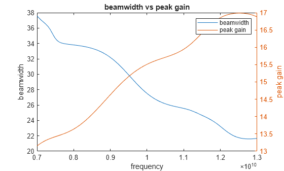
From the resulting plot, the inverse relationship between gain and beamwidth is clearly visible. Both analyses completed quickly for 101 frequency points, enabling efficient evaluation of the horn antenna's performance over a wide frequency range.
Analyze Surface Plot
Surface plots provide a powerful way to visualize how a horn antenna's performance varies with changes in its tunable geometric parameters. In this analysis, you examine how these parameters influence key performance metrics, including resonant frequency, bandwidth, peak gain, and beamwidth.
Vary each parameter within ±15% of its default value, and evaluate the performance metrics over a 20-by-20 grid of parameter combinations. Define the parameters for the surface plot.
L = antAI.defaultTunableParameters.FlareLength;
W = antAI.defaultTunableParameters.Width;
Flh = antAI.defaultTunableParameters.FlareHeight;
Fdh = antAI.defaultTunableParameters.FeedHeight;

npts = 20;
vScaler = linspace(0.85,1.15,npts);
Width vs Feed Height
Vary the Width and FeedHeight properties and calculate the resonant frequency, bandwidth, beamwidth and peak gain using the calcSurfResp function.
tic
[fResAI,bwAI,bmp1allAI,pgallAI] = calcSurfResp(W,Fdh,{'Width','FeedHeight'});
t1 = toc
t1 = 15.1765
Visualize the surface plots for the four analyses.
% Surface plot of Resonant Frequency
figure
subplot(2,2,1)
surf(W*vScaler,Fdh*vScaler,fResAI)
title("Resonant Frequency")
xlabel("Width")
ylabel("FeedHeight")
zlabel("fRes")
zlim([7e9,13e9])

% Surface plot of bandwidth
subplot(2,2,2);
surf(W*vScaler,Fdh*vScaler,bwAI)
title("Bandwidth")
xlabel("Width")
ylabel("FeedHeight")
zlabel("bandwidth")
zlim([1.2e9,4e9])

% Surface plot of beamwidth
subplot(2,2,3)
surf(W*vScaler,Fdh*vScaler,bmp1allAI)
title("Beamwidth")
xlabel("Width")
ylabel("FeedHeight")
zlabel("beamwidth")
zlim([24,36])

% Surface plot of peak gain
subplot(2,2,4);
surf(W*vScaler,Fdh*vScaler,pgallAI)
title("Peak Radiation")
xlabel("Width")
ylabel("FeedHeight")
zlabel("peak gain")
zlim([14,16])
hold off;
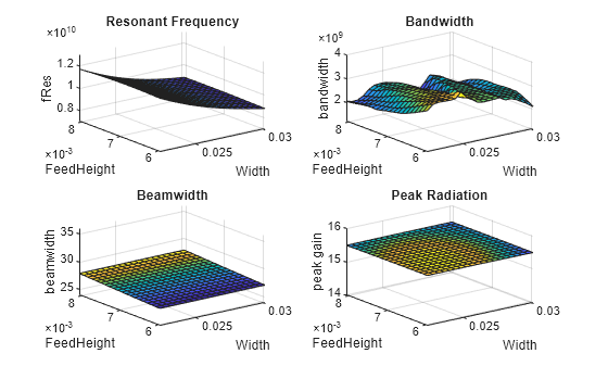
Width and feed height primarily affect the horn antenna's port analysis, resonant frequency, and bandwidth with width having a stronger influence. Their impact on field characteristics like peak gain and beamwidth is minimal, as these are more dependent on flare geometry.
Flare Length vs Flare Height
The FlareLength and FlareHeight properties define the horn's flare geometry and significantly influence peak gain and beamwidth by shaping the antenna's aperture and overall directivity. Vary the FlareLength and FlareHeight properties and perform all four analyses using the calcSurfResp function.
tic
[fResAI,bwAI,bmp1allAI,pgallAI] = calcSurfResp(L,Flh,{'FlareLength','FlareHeight'});
t2 = toc
t2 = 14.3578
% Surface plot of resonant frequency
figure
subplot(2,2,1)
surf(L*vScaler,Flh*vScaler,fResAI)
title("Resonant Frequency")
xlabel("FlareLength")
ylabel("FlareHeight")
zlabel("fRes")
zlim([7e9,13e9])

% Surface plot of bandwidth
subplot(2,2,2);
surf(L*vScaler,Flh*vScaler,bwAI)
title("Bandwidth")
xlabel("FlareLength")
ylabel("FlareHeight")
zlabel("bandwidth")
zlim([1.2e9,4e9])

% Surface plot of beamwidth
subplot(2,2,3)
surf(L*vScaler,Flh*vScaler,bmp1allAI)
title("beamwidth")
xlabel("FlareLength")
ylabel("FlareHeight")
zlabel("beamwidth")
zlim([24,36])


% Surface plot of peak gain
subplot(2,2,4);
surf(L*vScaler,Flh*vScaler,pgallAI)
title("Peak Radiation")
xlabel("FlareLength")
ylabel("FlareHeight")
zlabel("peak gain")
zlim([14,16])
hold off;
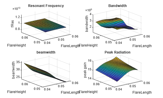
Flare length and flare height, play a crucial role in defining the horn antenna's radiation characteristics. Although these parameters have only a moderate effect on the resonant frequency, they significantly enhance bandwidth by improving impedance matching. More importantly, they are key to maximizing peak gain because they directly influence the aperture size and the resulting directivity. As flare length and flare height increase, peak gain improves and beamwidth narrows, demonstrating the classic tradeoff between directivity and coverage. This tradeoff makes flare geometry essential for applications that require high-gain, narrow-beam horn antennas.
Supporting Function
The calcSurfResp function calculates and returns the results of all four analyses by varying two tunable parameters over their entire range, 0.85 to 1.15 times the default value at the design frequency.
function [fResAI,bwAI,bmp1allAI,pgallAI] = calcSurfResp(V1,V2,var)
ant = horn;
f = 10e9;
antAI = design(ant,f,ForAI=true);

var1 = var{1};
var2 = var{2};

npts = 20;
vScaler = linspace(0.85,1.15,npts);

fResAI = zeros(npts);
bwAI = zeros(npts);
pgallAI = zeros(npts);
bmp1allAI = zeros(npts);


for i = 1:npts
    for j = 1:npts
        antAI.(var1) = V1*vScaler(i);
        antAI.(var2) = V2*vScaler(j);
        [~,~,~,matching] = bandwidth(antAI);
        switch string(matching)
            case "Matched"
                fResAI(i,j) = resonantFrequency(antAI);
                [bwAI(i,j),~,~] = bandwidth(antAI);
            case {"Almost","Not Matched"}
                fResAI(i,j) = NaN;
        end
        [pgallAI(i,j),~,~] = peakRadiation(antAI,f);
        [bm,~,~] = beamwidth(antAI,f);
        bmp1allAI(i,j) = bm(1,1);
    end
end
end
See Also
Objects
Functions
design|bandwidth|beamwidth|peakRadiation|resonantFrequency|exportAntenna|surf