Infinite Array of Microstrip Patch Antenna on Teflon Substrate

Define Unit Cell

A unit cell refers to a single element of an infinite array. This example uses a probe-fed microstrip patch element as a unit cell. The infinite array of a metal dielectric antenna must have a perfectlyconducting ground plane. Specify the ground plane length as 22.2 mm and width as 23.7 mm.

freq = 5e9;
vp = physconst('lightspeed');
lambda = vp/freq;
ucdx = 22.2e-3;
ucdy = 23.7e-3;

Create a probe-fed microstrip patch antenna with a lossy dielectric substrate.

elem = patchMicrostrip;
elem.Length = 18*1e-3;
elem.Width = 18*1e-3;
elem.Height = 1.59e-3;
elem.Substrate = dielectric('Teflon');
elem.Substrate.EpsilonR = 2.33;
elem.Substrate.LossTangent = 0.001;
elem.Substrate.Thickness = 1.59*1e-3;
elem.GroundPlaneLength = ucdx;
elem.GroundPlaneWidth = ucdy;
elem.FeedOffset = [9*1e-3-4.3e-3 0];

Create and Visualize Infinite Array

Create an infinite array and assign the probe-fed microstrip patch antenna as an element to the infinite array. Visualize the antenna.

ant = infiniteArray;
ant.Element = elem;
figure;
show(ant)

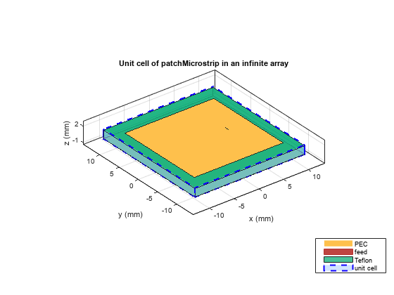
Visualize Current

In an Infinite array of metal dielectric structure with infinitely conductor backed dielectric substrate, only the upper metal layer is meshed. The impacts of dielectric and the infinite ground plane are considered in the dyadic Green's function. Calculate and visualize the current distribution on the top metal layer of the unit cell at the frequency of 5 GHz.

figure;
current(ant,freq)

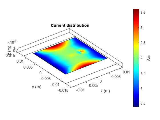
The current distribution looks similar to the standard dominant current distribution of a rectangular patch antenna with maxima near the two opposite edges.

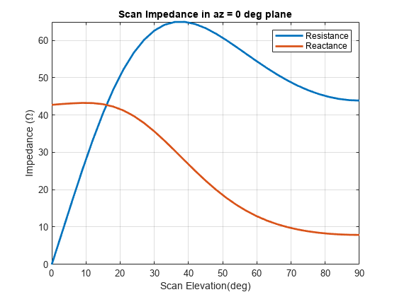
Compute and Visualize Scan Impedance

Compute and plot the scan impedance for varying elevation scan angles and a constant azimuth scan angle of zero degrees (E-plane). In an infinite array, the active reflection behavior and the scan element characteristics depend on the scan impedance behavior. For more information, see Infinite Array Analysis. As shown below, near the elevation angle of zero degrees the scan resistance is very low, indicating high reflection loss.

az = 0;            % aimuth, E-plane
el = 0:3:90;       % elevation
scanZ = nan(1,numel(el));
ant.ScanAzimuth = az;
for i = 1:numel(el)
    ant.ScanElevation = el(i);
    scanZ(i) = impedance(ant,freq);
end
figure
plot(el,real(scanZ),el,imag(scanZ),'LineWidth',2);
grid on
legend('Resistance','Reactance')
xlabel('Scan Elevation(deg)')
ylabel('Impedance (\Omega)')
title(['Scan Impedance in az = ' num2str(az) ' deg plane'])
axis tight

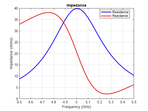
Scan Impedance and S-parameter Variation with Frequency

Fix the scan angles and sweep the frequency to observe the impedance behavior and the S-parameters of the unit cell element.

ant.ScanAzimuth = 0;
ant.ScanElevation = 90;
impedance(ant,linspace(4.5e9,5.5e9,31))

s=sparameters(ant,linspace(4.5e9,5.5e9,31));
figure;
rfplot(s,1,1)

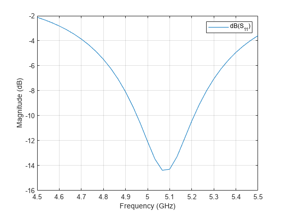
The port reflection shows a dip of around 5.1 GHz, which closely matches the results in [1].

Reference

[1] Deshpande, M., and P. Prabhakar. “Analysis of Dielectric Covered Infinite Array of Rectangular Microstrip Antennas.” IEEE Transactions on Antennas and Propagation 35, no. 6 (June 1987): 732–36. https://doi.org/10.1109/TAP.1987.1144169.