Ray Tracing for Wireless Communications

Introduction

Wireless communication systems use radio waves to transmit signals. Propagation modeling enables you to estimate the strength of signals based on system parameters such as frequency, antenna height, terrain properties, and building properties.

Theoretical and empirical models estimate path loss based on range, and are valid only for those environments that resemble the modeling environment. As a result, these models usually do not provide accurate temporal or spatial information. Unlike these models, ray tracing models are specific to the 3-D environment, and are therefore appropriate for scenarios such as urban environments.

For propagation modeling, a ray is an individual radio signal that [1]:

Travels in a straight line through a homogeneous medium.
Obeys the laws of reflection, refraction, and diffraction.
Carries energy. Propagation models treat rays like tubes, where the energy density on the cross section becomes smaller as the ray interacts with the environment.

For a given 3-D environment, ray tracing models use numerical simulations to:

Predict the paths of rays from transmitters to receivers. The models can find many rays from a transmitter to a receiver. The models derive the angle of departure, angle of arrival, and time of arrival from the paths.
Estimate the path loss and phase change for each ray. Total path loss is the sum of interaction losses, free space loss, and, optionally, atmospheric loss.

A ray interacts with the environment in several ways [1].

Interaction	Description
Line of sight (LOS)	The ray travels directly from the transmitter to the receiver.
Reflection	The ray reflects off a surface according to the law of reflection.
Refraction (transmission)	The ray refracts as it moves into a new medium, according to the law of refraction.
Diffraction	The ray diffracts off a surface according to the law of diffraction. One ray can spawn many diffracted rays.
Diffuse scattering	The ray interacts with a rough surface such as the ocean or a building facade.

Use these functions to create ray tracing models, predict propagation paths, and calculate path losses and phase shifts.

propagationModel — Create a ray tracing model as a RayTracing object. Specify options such as the ray tracing method, the maximum number of reflections and diffractions, and the interaction materials. You can use ray tracing models as inputs when conducing RF analysis, such as when generating coverage maps by using the coverage function or when calculating total received power by using the sigstrength function.
raytrace — Display propagation paths (rays) on a map or return propagation paths as comm.Ray objects. Each object represents the full path from the transmitter to the receiver, and contains information such as the path loss, phase shift, and types of surface interactions.
raypl — Calculate the path loss and phase shift for a propagation path based on surface materials and antenna polarization types.

For an example that shows ray tracing in an urban environment, see Urban Link and Coverage Analysis Using Ray Tracing.

Ray Tracing Methods

The propagationModel and raytrace functions use a ray tracing model that finds LOS and non-line-of-sight (NLOS) paths.

The model finds LOS paths by shooting a ray from the transmitter toward the receiver. If the ray does not interact with a surface before reaching the receiver, then an LOS path exists.
The model finds NLOS paths by using either the shooting and bouncing rays (SBR) method [2] or the image method. You can specify the method by using the propagationModel function.

Choose a method based on the types of interactions you want to model, the computation speed, and the accuracy.

Method	Interaction Types	Computation Speed	Computation Accuracy
SBR (the default)	Includes effects from reflection and edge diffraction. Does not include effects from corner diffraction, refraction, or diffuse scattering. For each path, supports up to ten path reflections and two edge diffractions.	Computational complexity increases linearly with the number of reflections and exponentially with the number of diffractions. The SBR method is generally faster than the image method.	Calculates an approximate number of propagation paths with exact geometric accuracy.
Image	Includes effects from reflection. Does not include effects from diffraction, refraction, or diffuse scattering. For each path, supports up to two path reflections.	Computational complexity increases exponentially with the number of reflections.	Calculates an exact number of propagation paths with exact geometric accuracy.

Method

Interaction Types

Computation Speed

Computation Accuracy

SBR (the default)

Includes effects from reflection and edge diffraction. Does not include effects from corner diffraction, refraction, or diffuse scattering.

For each path, supports up to ten path reflections and two edge diffractions.

Computational complexity increases linearly with the number of reflections and exponentially with the number of diffractions. The SBR method is generally faster than the image method.

Calculates an approximate number of propagation paths with exact geometric accuracy.

Image

Includes effects from reflection. Does not include effects from diffraction, refraction, or diffuse scattering.

For each path, supports up to two path reflections.

Computational complexity increases exponentially with the number of reflections.

Calculates an exact number of propagation paths with exact geometric accuracy.

When both the image and SBR methods find the same path, the points along the path are the same within a tolerance of machine precision for single-precision floating-point values.

SBR Method

This figure illustrates the SBR method for calculating propagation paths from a transmitter, Tx, to a receiver, Rx.

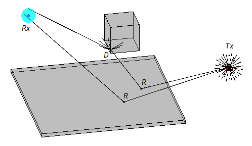
$Ray tracing reflection and diffraction using the SBR method$

The SBR method launches many rays from a geodesic sphere centered at Tx. The geodesic sphere enables the model to launch rays that are approximately uniformly spaced.

Then, the method traces every ray from Tx and can model different types of interactions between the rays and surrounding objects, such as reflections, diffractions, refractions, and scattering. Note that the current implementation of the SBR method considers only reflections and edge diffractions.

When a ray hits a flat surface, shown as R, the ray reflects based on the law of reflection.
When a ray hits an edge, shown as D, the ray spawns many diffracted rays based on the law of diffraction [3][4]. Each diffracted ray has the same angle with the diffracting edge as the incident ray. The diffraction point then becomes a new launching point and the SBR method traces the diffracted rays in the same way as the rays launched from Tx. A continuum of diffracted rays forms a cone around the diffracting edge, which is commonly known as a Keller cone [4].

For each launched ray, the SBR method surrounds Rx with a sphere, called a reception sphere, with a radius that is proportional to the distance the ray travels and the average number of degrees between the launched rays. If the ray intersects the sphere, then the model considers the ray a valid path from Tx to Rx. The SBR method corrects the valid paths so that the paths have exact geometric accuracy.

When you increase the number of rays by decreasing the number of degrees between rays, the reception sphere becomes smaller. As a result, in some cases, launching more rays results in fewer or different paths. This situation is more likely to occur with custom 3-D scenarios created from STL files or triangulation objects than with scenarios that are automatically generated from OpenStreetMap^® buildings and terrain data.

The SBR method finds paths using double-precision floating-point computations.

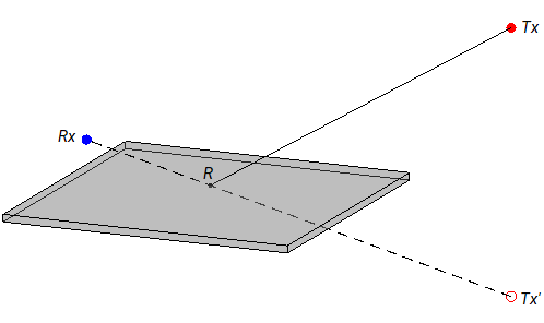
Image Method

This figure illustrates the image method for calculating the propagation path of a single reflection ray for the same transmitter and receiver as the SBR method. The image method locates the image of Tx with respect to a planar reflection surface, Tx'. Then, the method connects Tx' and Rx with a line segment. If the line segment intersects the planar reflection surface, shown as R in the figure, then a valid path from Tx to Rx exists. The method determines paths with multiple reflections by recursively extending these steps. The image method finds paths using single-precision floating-point computations.

Ray tracing using the image method

Propagation Loss

RayTracing objects calculate reflection and diffraction losses by tracking the horizontal and vertical polarizations of signals through the propagation path. Total power loss is the sum of free space loss, reflection loss, and diffraction loss.

Effect of Surface Materials

When a ray interacts with a surface, the surface material impacts the reflection losses.

The ray tracing model incorporates building and surface materials into the propagation loss calculations by using the complex relative permittivity of the surface, ε_r. The ITU-R P.2040-3 [5] and ITU-R P.527-5 through ITU-R P.527-6 [6] recommendations include methods, equations, and values used to calculate ε_r for a range of frequencies.

The equations for ε_r are:

$ε_{r} = ε_{r}^{'} + j ε_{r}^{' '}$

$ε_{r}^{' '} = \frac{σ}{2 π ε_{0} f}$ ,

where:

ε_r' is the real relative permittivity.
σ is the conductivity in S/m.
ε₀ is the permittivity of free space (electric constant).
f is the frequency in Hz.

For building materials, the ray tracing model calculates ε_r' and σ as:

$ε_{r}^{'} = a f^{b}$

$σ = c f^{d}$ ,

where a, b, c, and d are constants determined by the surface material. For readability, this table shows the frequency range in GHz.

Material Class	Real Part of Relative Permittivity		Conductivity (S/m)		Frequency Range (GHz)
Material Class	a	b	c	d	Frequency Range (GHz)
Vacuum (~ air)	1	0	0	0	[0.001, 100]
Concrete	5.24	0	0.0462	0.7822	[1, 100]
Brick	3.91	0	0.0238	0.16	[1, 10]
Plasterboard	2.73	0	0.0085	0.9395	[1, 100]
Wood	1.99	0	0.0047	1.0718	[0.001, 100]
Glass	6.31	0	0.0036	1.3394	[0.1, 100]
Glass	5.79	0	0.0004	1.658	[220, 450]
Ceiling board	1.48	0	0.0011	1.0750	[1, 100]
Ceiling board	1.52	0	0.0029	1.029	[220, 450]
Chipboard	2.58	0	0.0217	0.78	[1, 100]
Plywood	2.71	0	0.33	0	[1, 40]
Marble	7.074	0	0.0055	0.9262	[1, 60]
Floorboard	3.66	0	0.0044	1.3515	[50, 100]
Metal	1	0	10⁷	0	[1, 100]
Very dry ground	3	0	0.00015	2.52	[1, 10] only^(a)
Medium dry ground	15	– 0.1	0.035	1.63	[1, 10] only^(a)
Wet ground	30	– 0.4	0.15	1.30	[1, 10] only^(a)
Note (a): For the three ground types (very dry, medium dry, and wet), you cannot exceed the noted frequency limits.

For earth surfaces such as water, sea water, pure or wet ice, dry or wet soil, and vegetation, the ray tracing model calculates ε_r using the methods and equations presented in ITU-R P.527-5 through ITU-R P.527-6 [6].

Reflection Loss

This image shows a reflection path from a transmitter site tx to a receiver site rx.

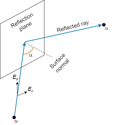
Reflection path from a transmitter site to a receiver site

The model determines polarization and reflection loss using these steps.

Track the propagation of the ray in 3-D space by calculating the propagation matrix P. The matrix is a repeating product, where i is the number of reflection points.
$P = \prod_{i} P_{i}$
For each reflection, calculate P_i by transforming the global coordinates of the incident electromagnetic field into the local coordinates of the reflection plane, multiplying the result by a reflection coefficient matrix, and transforming the coordinates back into the original global coordinate system [7]. The equations for P_i and P₀ are:

$P_{i} = \begin{matrix} {[\begin{matrix} s_{o u t} & p_{o u t} & k_{o u t} \end{matrix}]}_{i} & {[\begin{matrix} R_{V} (α) & 0 & 0 \\ 0 & R_{H} (α) & 0 \\ 0 & 0 & 1 \end{matrix}]}_{i} & {[\begin{matrix} s_{i n} & p_{i n} & k_{i n} \end{matrix}]}_{i}^{- 1} \end{matrix}$

$P_{0} = [\begin{matrix} 1 & 0 & 0 \\ 0 & 1 & 0 \\ 0 & 0 & 1 \end{matrix}]$
where:
- s, p, and k form a basis for the plane of incidence (the plane created by the incident ray and the surface normal of the reflection plane). s and p are perpendicular and parallel, respectively, to the plane of incidence.
- k_in and k_out are the directions (in global coordinates) of the incident and exiting rays, respectively.
- s_in and s_out are the directions (in global coordinates) of the horizontal polarizations for the incident and exiting rays, respectively.
- p_in and p_out are the directions (in global coordinates) of the vertical polarizations for the incident and exiting rays, respectively.
- R_H and R_V are the Fresnel reflection coefficients for the horizontal and vertical polarizations, respectively. α is the incident angle of the ray and ε_r is the complex relative permittivity of the material.
  $R_{H} (α) = \frac{\cos (α) - \sqrt{(ε_{r} - \sin^{2} (α)) / ε_{r}^{2}}}{\cos (α) + \sqrt{(ε_{r} - \sin^{2} (α)) / ε_{r}^{2}}}$
  $R_{V} (α) = \frac{\cos (α) - \sqrt{ε_{r} - \sin^{2} (α)}}{\cos (α) + \sqrt{ε_{r} - \sin^{2} (α)}}$
Project the propagation matrix P into a 2-by-2 polarization matrix R. The model rotates the coordinate systems for the transmitter and receiver so that they are in global coordinates.
$R = [\begin{matrix} H_{i n} \cdot H_{r x} & V_{i n} \cdot H_{r x} \\ H_{i n} \cdot V_{r x} & V_{i n} \cdot V_{r x} \end{matrix}]$
$H_{i n} = P (V_{t x} \times k_{t x})$
$V_{i n} = P V_{t x}$
where:
- H_rx and V_rx are the directions (in global coordinates) of the horizontal (E_θ) and vertical (E_ϕ) polarizations, respectively, for the receiver.
- H_in and V_in are the directions (in global coordinates) of the propagated horizontal and vertical polarizations, respectively.
- V_tx is the direction (in global coordinates) of the nominal vertical polarization for the ray departing the transmitter.
- k_tx is the direction (in global coordinates) of the ray departing the transmitter.
Specify the normalized horizontal and vertical polarizations of the electric field at the transmitter and receiver by using the 2-by-1 Jones polarization vectors J_tx and J_rx, respectively. If either the transmitter or receiver are unpolarized, then the model assumes $J_{t x} = J_{r x} = \frac{\sqrt{2}}{2} [\begin{matrix} 1 \\ 1 \end{matrix}]$ .
Calculate the polarization and reflection loss IL by combining R, J_tx, and J_rx.
$I L = - 20 \log_{10} | J_{r x}^{- 1} R J_{t x} |$

Diffraction Loss

The model calculates diffraction loss by using computations based on the Uniform Theory of Diffraction (UTD) [8].

For a first order signal diffraction, the equation for path loss, PL_D, is:

$P L_{D} = J V_{r x}^{'} H_{d i f f 1} J V_{t x}$ ,

where:

JV_rx and JV_tx are polarization vectors for the receiver and transmitter, respectively, specified as Jones vectors.
H_diff1 is the diffraction matrix.

The equation for the diffraction matrix contains three terms.

The first term is a geometric coupling matrix that rotates the polarization vector from the basis of the ray coordinates to the basis of the edge-fixed incidence plane. The edge-fixed incidence plane contains the ray and the edge.
The second term is a polarization matrix containing diffraction coefficients for the local horizontal and vertical polarizations, D_⟂ and D_∥, and an amplitude scaling factor. For more information about the diffraction coefficients and amplitude scaling factor, see [3] and [8].
The third term is a geometric coupling matrix that rotates the polarization vector from the basis of the edge-fixed incidence plane to the basis of the edge-fixed diffraction plane. The edge-fixed diffraction plane contains the diffracted ray and the edge.

References

[1] Yun, Zhengqing, and Magdy F. Iskander. “Ray Tracing for Radio Propagation Modeling: Principles and Applications.” IEEE Access 3 (2015): 1089–1100. https://doi.org/10.1109/ACCESS.2015.2453991.

[2] Schaubach, K.R., N.J. Davis, and T.S. Rappaport. “A Ray Tracing Method for Predicting Path Loss and Delay Spread in Microcellular Environments.” In [1992 Proceedings] Vehicular Technology Society 42nd VTS Conference - Frontiers of Technology, 932–35. Denver, CO, USA: IEEE, 1992. https://doi.org/10.1109/VETEC.1992.245274.

[3] International Telecommunications Union Radiocommunication Sector. Propagation by diffraction. Recommendation P.526-15. ITU-R, approved October 21, 2019. https://www.itu.int/rec/R-REC-P.526/en.

[4] Keller, Joseph B. “Geometrical Theory of Diffraction.” Journal of the Optical Society of America 52, no. 2 (February 1, 1962): 116. https://doi.org/10.1364/JOSA.52.000116.

[5] International Telecommunications Union Radiocommunication Sector. Effects of Building Materials and Structures on Radiowave Propagation Above About 100MHz. Recommendation P.2040. ITU-R, approved August 23, 2023. https://www.itu.int/rec/R-REC-P.2040/en.

[6] International Telecommunications Union Radiocommunication Sector. Electrical Characteristics of the Surface of the Earth. Recommendation P.527. ITU-R, approved September 27, 2021. https://www.itu.int/rec/R-REC-P.527/en.

[7] Chipman, Russell A., Garam Young, and Wai Sze Tiffany Lam. "Fresnel Equations." In Polarized Light and Optical Systems. Optical Sciences and Applications of Light. Boca Raton: Taylor & Francis, CRC Press, 2019.

[8] McNamara, D. A., C. W. I. Pistorius, and J. A. G. Malherbe. Introduction to the Uniform Geometrical Theory of Diffraction. Boston: Artech House, 1990.