Train Machine Learning Model for Analysis of Custom Antenna
This example demonstrates how to apply machine learning to antenna analysis and illustrates a general recipe that you can use to train machine learning models to characterize antenna structures modeled and simulated in Antenna Toolbox™.
Overview of Machine Learning Workflow for Antenna Analysis
The overall workflow entails the following steps:
Model and parameterize the antenna structure in Antenna Toolbox.
Identify the tunable design variables (predictors) and analysis metrics (responses) for the machine learning model to learn.
Conduct a design of experiments (DOE) to get a representative collection of observations comprised of values for the design variables sampled within the ranges of interest.
Generate response data using full-wave simulation of the antenna for each parameter set.
Prepare and preprocess the data for training, tuning, and testing candidate machine learning models.
Iteratively train and optimize hyperparameters across various machine learning models to select an optimal model that has good predictive performance.
Assess the model's performance and prediction accuracy against full-wave simulation results.
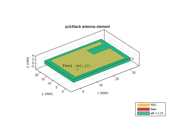
In this example, the antenna of interest is the C-shaped microstrip patch antenna. As per [1] and [2], this antenna is constructed by cutting a rectangular slot at a radiating edge of a conventional rectangular patch antenna. The analysis metric of interest is the resonant frequency, defined here as the operating frequency at which the reflection coefficient magnitude () is minimum. This example follows [2] and [3] in its adoption of the -based definition of resonant frequency. This is in contrast to the impedance-based definition, which defines the resonant frequency as the frequency at which the reactance is equal to zero, as adopted in [4].
Model and Parameterize Custom Antenna Structure
Define Parameter Sets for Antenna Design Variables
Specify the number of predictors, which correspond to the tunable design variables for the antenna.
numpreds = 7;
Define the combinations of antenna design parameters as provided in [2]. In this example, there are five pairs of length and width values. For each pair, there are two possible slot lengths, two possible slot widths, and two possible slot offsets. This yields 5×2×2×2 = 40 configurations. For each of these configurations, there are two possible substrate heights and two possible dielectric constants. This yields a total of 40×2×2 = 160 antenna parameter sets. Note that the geometric parameters here are all specified in millimeters.
Lp = [30; 35; 40; 45; 50];                % Length (mm)
Wp = [20; 25; 30; 35; 40];                % Width (mm)
ls = [10 20; 15 25; 15 30; 25 30; 20 40]; % Slot length (mm)
ws = [5 10; 7 12; 7.5 15; 5 10; 10 20];   % Slot width (mm)
ds = [3 6; 8 10; 5 10; 20 25; 7 14];      % Slot offset (mm)
h = [1.6 2.5];                            % Substrate height (mm)
eR = [2.33 4.4];                          % Substrate relative permittivity
View the sets of patch dimensions in table format to elucidate the correspondence between the sets of outer dimensions and the respective choices of slot dimensions.
disp(table(Lp,Wp,ls,ws,ds))
    Lp    Wp       ls           ws           ds
    __    __    ________    __________    ________

    30    20    10    20      5     10     3     6
    35    25    15    25      7     12     8    10
    40    30    15    30    7.5     15     5    10
    45    35    25    30      5     10    20    25
    50    40    20    40     10     20     7    14
Define Fixed Parameters for Antenna Feed
Specify the feed location in meters and the feed excitation voltage.
feedparams.x0 = 5e-3; % m
feedparams.y0 = 5e-3; % m
feedparams.V = 1;     % V
Examine Antenna Structure
Use the helper function, createCShapedPatchAntenna, to create a PCB stack model of the antenna for the first of the 160 parameter sets. When calling the helper function, set Visualize=true to view the antenna's structure and parameterization. For all parameter sets in this example, the helper function specifies the ground plane dimensions as 1.15 times the respective outer dimensions of the radiating patch.
ant = createCShapedPatchAntenna( ...
    Lp(1),Wp(1),ls(1,1),ws(1,1),ds(1,1),h(1),eR(1), ...
    feedparams,Visualize=true);

Create Full Factorial Design to Assemble Table of Antenna Design Parameter Sets
Generate a full factorial design to account for the 160 antenna parameter configurations. Full factorial design is one type of DOE technique. In this example, the parameter combinations have been preselected from [2] as a representative distribution composed of discrete sets of values for each parameter. Accordingly, a full factorial design from the curated parameter sets is appropriate. Note that other DOE techniques exist to perform data collection in a parsimonious manner and/or from a continuous distribution of parameter values, as shown in [4]. For more information, see Design of Experiments (DOE) (Statistics and Machine Learning Toolbox).
dFF = fullfact([5 2 2 2 2 2])
dFF = 160×6

     1     1     1     1     1     1
     2     1     1     1     1     1
     3     1     1     1     1     1
     4     1     1     1     1     1
     5     1     1     1     1     1
     1     2     1     1     1     1
     2     2     1     1     1     1
     3     2     1     1     1     1
     4     2     1     1     1     1
     5     2     1     1     1     1
     1     1     2     1     1     1
     2     1     2     1     1     1
     3     1     2     1     1     1
     4     1     2     1     1     1
     5     1     2     1     1     1
      ⋮
N = height(dFF)
N =
160
The structure of dFF, the full factorial design matrix, is as follows:
The first column of
dFFcontains the indices for the sets of outer dimensions, namely the length (Lp) and the width (Wp) values.The second, third, and fourth columns of
dFFcontain the indices to specify the choice of slot dimensions, namely the slot length (ls), slot width (ws), and slot offset (ds), respectively, corresponding to the choice of outer dimensions. In particular, when indexing intols,ws, andds, use the first column ofdFFto adhere to the correspondence between the combinations of slot dimensions and the sets of outer dimensions.The fifth and sixth columns of
dFFcontain the indices for the sets of substrate height (h) and relative permittivity (eR) values, respectively.
Use this full factorial design to construct a table of predictor values. For completeness, capture the units for the predictor variables in the table properties.
T0 = array2table(zeros(N,numpreds), ...
    VariableNames=["Lp","Wp","ls","ws","ds","h","eR"],RowNames=string(1:N));

for idx = 1:N
    rowIdx = dFF(idx,1);

    T0.Lp(idx) = Lp(rowIdx);
    T0.Wp(idx) = Wp(rowIdx);

    T0.ls(idx) = ls(rowIdx,dFF(idx,2));
    T0.ws(idx) = ws(rowIdx,dFF(idx,3));
    T0.ds(idx) = ds(rowIdx,dFF(idx,4));

    T0.h(idx) = h(dFF(idx,5));
    T0.eR(idx) = eR(dFF(idx,6));
end

T0.Properties.VariableUnits = ["mm","mm","mm","mm","mm","mm",""]
T0=160×7 table
          Lp    Wp    ls    ws     ds     h      eR
          __    __    __    ___    __    ___    ____

    1     30    20    10      5     3    1.6    2.33
    2     35    25    15      7     8    1.6    2.33
    3     40    30    15    7.5     5    1.6    2.33
    4     45    35    25      5    20    1.6    2.33
    5     50    40    20     10     7    1.6    2.33
    6     30    20    20      5     3    1.6    2.33
    7     35    25    25      7     8    1.6    2.33
    8     40    30    30    7.5     5    1.6    2.33
    9     45    35    30      5    20    1.6    2.33
    10    50    40    40     10     7    1.6    2.33
    11    30    20    10     10     3    1.6    2.33
    12    35    25    15     12     8    1.6    2.33
    13    40    30    15     15     5    1.6    2.33
    14    45    35    25     10    20    1.6    2.33
    15    50    40    20     20     7    1.6    2.33
    16    30    20    20     10     3    1.6    2.33
      ⋮
Generate Data Using Full-Wave Simulation
Define Simulation Parameters for Antenna Port Analysis
Specify the simulation frequency sweep across which to compute the antenna's frequency response: 1–5 GHz with a resolution of 50 MHz.
f = 1e9:50e6:5e9;
Generate Raw Data for S-Parameter and Impedance Frequency Responses
You can load the pregenerated data set from the file, CShapedPatchAntennaS11Data.zip, that is included with this example, or you can regenerate the data using the generateObservation helper function. In the latter case, you can optionally parallelize the data generation process if you have a Parallel Computing Toolbox™ license. Note that data regeneration can take several hours to complete. For each observation, the generateObservation helper function first calls the createCShapedPatchAntenna helper function to create the antenna structure and then performs full-wave simulation to compute the complex-valued S-parameter response over the frequency sweep specified by f. Use the interactive drop-down controls in this example to modify the data generation settings.
S = cell(N,1); switch"LoadGeneratedData" case "LoadGeneratedData" foldername = "data"; if ~isfolder(foldername) unzip CShapedPatchAntennaS11Data.zip end files = dir(fullfile(foldername,"*.mat")); for idx = 1:N filename = files(idx).name; data = load(fullfile(foldername,filename),"S"); S{idx} = data.S; end case "RegenerateData" if
false parfor idx = 1:N [S{idx},~] = generateObservation(T0(idx,:),feedparams,f, ... SaveDataToFile=
true,FileIndex=idx); end else for idx = 1:N [S{idx},~] = generateObservation(T0(idx,:),feedparams,f, ... SaveDataToFile=
true,FileIndex=idx); end end end
Perform Feature Extraction to Obtain Resonant Frequency Values from Raw Data
As per [2] and [3], search for resonances within 1.15–3.335 GHz, as the antenna parameter ranges are selected for ultra-high frequency (UHF) applications.
jdx = find(f >= 1.15e9 & f <= 3.335e9);
fs = f(jdx);
In particular, look for local minima in the responses within the 1.15–3.335 GHz frequency range. For each antenna, select the lowest frequency corresponding to an local minimum as the resonant frequency of interest, as this corresponds to the fundamental resonance.
fR = zeros(N,1);
for idx = 1:N
    S11 = S{idx}.Parameters;
    S11 = 20*log10(abs(S11));
    S11 = S11(jdx);
    kdx = find(islocalmin(S11),1);
    fR(idx) = fs(kdx);
end
Prepare and Preprocess Data for Training and Testing
Assemble Predictor and Response Data into Table Format
Rescale the resonant frequency values to units of GHz, and then add them to the table as the response data.
T = addvars(T0,fR/1e9,NewVariableNames="fR");
T.Properties.VariableUnits(end) = "GHz"
T=160×8 table
          Lp    Wp    ls    ws     ds     h      eR      fR
          __    __    __    ___    __    ___    ____    ____

    1     30    20    10      5     3    1.6    2.33     3.2
    2     35    25    15      7     8    1.6    2.33    2.25
    3     40    30    15    7.5     5    1.6    2.33     2.5
    4     45    35    25      5    20    1.6    2.33    1.45
    5     50    40    20     10     7    1.6    2.33     1.6
    6     30    20    20      5     3    1.6    2.33     2.1
    7     35    25    25      7     8    1.6    2.33    1.55
    8     40    30    30    7.5     5    1.6    2.33    1.35
    9     45    35    30      5    20    1.6    2.33    1.25
    10    50    40    40     10     7    1.6    2.33    1.85
    11    30    20    10     10     3    1.6    2.33     3.1
    12    35    25    15     12     8    1.6    2.33    2.25
    13    40    30    15     15     5    1.6    2.33     2.1
    14    45    35    25     10    20    1.6    2.33     1.5
    15    50    40    20     20     7    1.6    2.33    1.55
    16    30    20    20     10     3    1.6    2.33       2
      ⋮
Visualize and Explore Distribution of Data
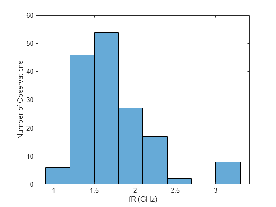
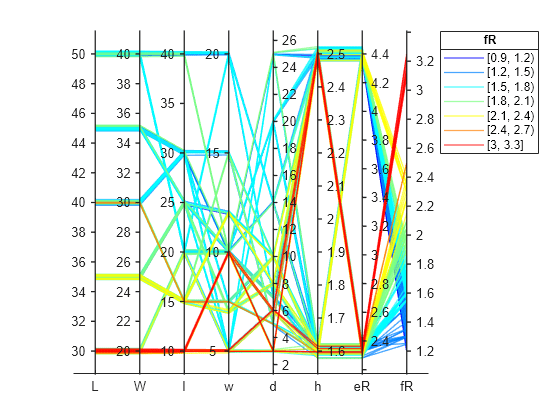
Data examination and visualization comprise an important step in a machine learning workflow. Visually explore the data to understand its structure and distribution. This can help you assess the quality of the collected data set and familiarize with the overarching relationships therein. It can also help you assess, compare, interpret, and/or contextualize the predictions eventually made by the trained models. This example presents two such visualization tools: histogram plots and parallel coordinates plots. For more information about these and other visualization tools, see Data Distribution Plots and Statistical Visualization (Statistics and Machine Learning Toolbox).
Create Histogram Plot
Create a histogram plot with automatic binning to understand the overall distribution of the response data.
figure
hhist = histogram(T.fR);
xlabel("fR (GHz)")
ylabel("Number of Observations")
Create Parallel Coordinates Plot
Create a parallel coordinates plot from the table, T, to visualize the multivariate relationships present in the data. Use the discretize function to bin the response values according to the bins automatically selected by the histogram function. Append the set of binned response values to the source table of the parallel coordinates plot, sort this source table according to the binning, and then group and color code the lines in the plot accordingly. Use the jet colormap to assign a distinct color to each binned group.
figure
hpcplot = parallelplot(T,CoordinateVariables=1:width(T));
fR_group = discretize(T.fR,hhist.BinEdges,"categorical");
hpcplot.SourceTable.fR_group = fR_group;
hpcplot.SourceTable = sortrows(hpcplot.SourceTable, ...
    ["fR_group","Lp","Wp","ls","ws","ds","h","eR"]);
hpcplot.GroupVariable = "fR_group";
hpcplot.LegendTitle = "fR";
hpcplot.Color = jet(hhist.NumBins);
Partition Data into Training and Test Sets
Use cvpartition with the Holdout parameter to randomly partition the data into a training set containing 80% of the observations and a test set containing 20% of the observations. Use the former to train and tune the machine learning model, and use the latter to test the performance of the trained model on new data. Stratify the partition according to the binning groups in fR_group to balance the response distribution across the training and test data sets and to achieve consistency of each with the distribution of the overall data. For the sake of reproducibility, set the random number generator seed to 1.
rng(1)
partition = cvpartition(fR_group,HoldOut=0.2,Stratify=true);
idxTrain = training(partition);
idxTest = test(partition);
dataTrain = T(idxTrain,:)
dataTrain=130×8 table
          Lp    Wp    ls    ws     ds     h      eR      fR
          __    __    __    ___    __    ___    ____    ____

    1     30    20    10      5     3    1.6    2.33     3.2
    2     35    25    15      7     8    1.6    2.33    2.25
    4     45    35    25      5    20    1.6    2.33    1.45
    5     50    40    20     10     7    1.6    2.33     1.6
    6     30    20    20      5     3    1.6    2.33     2.1
    8     40    30    30    7.5     5    1.6    2.33    1.35
    9     45    35    30      5    20    1.6    2.33    1.25
    10    50    40    40     10     7    1.6    2.33    1.85
    11    30    20    10     10     3    1.6    2.33     3.1
    12    35    25    15     12     8    1.6    2.33    2.25
    13    40    30    15     15     5    1.6    2.33     2.1
    14    45    35    25     10    20    1.6    2.33     1.5
    15    50    40    20     20     7    1.6    2.33    1.55
    16    30    20    20     10     3    1.6    2.33       2
    17    35    25    25     12     8    1.6    2.33    1.55
    19    45    35    30     10    20    1.6    2.33     1.3
      ⋮
dataTest = T(idxTest,:)
dataTest=30×8 table
           Lp    Wp    ls    ws     ds     h      eR      fR
           __    __    __    ___    __    ___    ____    ____

    3      40    30    15    7.5     5    1.6    2.33     2.5
    7      35    25    25      7     8    1.6    2.33    1.55
    18     40    30    30     15     5    1.6    2.33     1.3
    24     45    35    25      5    25    1.6    2.33     1.6
    39     45    35    30     10    25    1.6    2.33       2
    40     50    40    40     20    14    1.6    2.33    1.75
    41     30    20    10      5     3    2.5    2.33    3.25
    44     45    35    25      5    20    2.5    2.33     1.5
    56     30    20    20     10     3    2.5    2.33    2.05
    58     40    30    30     15     5    2.5    2.33     1.3
    59     45    35    30     10    20    2.5    2.33     1.3
    62     35    25    15      7    10    2.5    2.33    2.25
    73     40    30    15     15    10    2.5    2.33     2.1
    87     35    25    25      7     8    1.6     4.4     1.9
    98     40    30    30     15     5    1.6     4.4     1.6
    103    40    30    15    7.5    10    1.6     4.4     1.5
      ⋮
Examine Distribution of Response Values of Training vs. Test Data
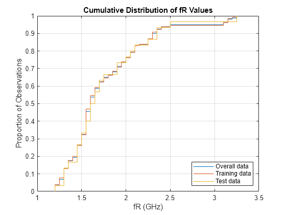
It is important for the training data set to be statistically representative of the overall data so as not to bias or skew the model from learning how to generalize. It is also important for the test data set to be statistically similar to the training data set. Otherwise, the model's performance on the test data may not be a good indicator of the model's ability to generalize to new data drawn from the same population.
Compare the distribution of the response values in the training vs. test data sets to assess the degree of parity between the two. This example presents three visualization tools to perform this comparison: box plots, cumulative distribution plots, and histogram plots.
Create Box Plots
Create box charts of the response values from the overall data, training data, and test data.
figure
htlb = tiledlayout(1,3);
title(htlb,"Response Distribution")
ylabel(htlb,"fR (GHz)")

nexttile
boxchart(T.fR)
title("Overall Data")
ylim([1 3.5])

nexttile
boxchart(dataTrain.fR)
title("Training Data")
ylim([1 3.5])

nexttile
boxchart(dataTest.fR)
title("Test Data")
ylim([1 3.5])

Create Cumulative Distribution Plots
Create cumulative distribution plots of the response values from the overall data, training data, and test data.
figure
cdfplot(T.fR)
hold on
cdfplot(dataTrain.fR)
cdfplot(dataTest.fR)
hold off
xlabel("fR (GHz)")
ylabel("Proportion of Observations")
title("Cumulative Distribution of fR Values")
legend("Overall data","Training data","Test data",Location="southeast")
Create Histogram Plots
Create histograms of the response values from the overall data, training data, and test data. Use the same bin edges and normalization method across all plots.
figure
htlh = tiledlayout(1,3);
title(htlh,"Response Distribution")
xlabel(htlh,"fR (GHz)")
ylabel(htlh,"Proportion of Observations")

nexttile
histogram(T.fR,BinEdges=hhist.BinEdges,Normalization="probability")
title("Overall data")

nexttile
histogram(dataTrain.fR,BinEdges=hhist.BinEdges,Normalization="probability")
title("Training data")

nexttile
histogram(dataTest.fR,BinEdges=hhist.BinEdges,Normalization="probability")
title("Test data")

Use AutoML to Automatically Select and Train Regression Model with Optimized Hyperparameters
Statistics and Machine Learning Toolbox™ supports automated machine learning (AutoML) capabilities to automate, accelerate, and streamline the iterative process of model selection, configuration, hyperparameter tuning, optimization, examination, and visualization. This example focuses on the command-line workflow using the fitrauto (Statistics and Machine Learning Toolbox) function to automatically train and tune a selection of regression model types and hyperparameter values. That said, the software also supports interactive workflows within the Regression Learner App (Statistics and Machine Learning Toolbox). Refer to the following pages for more information:
Automated Regression Model Selection with Bayesian and ASHA Optimization (Statistics and Machine Learning Toolbox)
Train Regression Models in Regression Learner App (Statistics and Machine Learning Toolbox)
Train Model Using fitrauto
Use the fitrauto function to iteratively train and tune a variety of regression model types. The distribution of the training data suggests that a nonlinear model is more suitable than a linear model. Accordingly, set the Learners parameter to instruct fitrauto to consider only the following nonlinear types of models: Gaussian process, kernel, neural network, and support vector machine regression models.
In this example, use fitrauto with its default optimization algorithm, Bayesian Optimization (Statistics and Machine Learning Toolbox). In addition, you can customize the hyperparameter optimization options.
Set
MaxObjectiveEvaluationsto60to limit the number of iterations and indirectly limit the runtime. Otherwise, the software defaults to 30 iterations per learner, which in this case is 30×4 = 120 iterations. Alternatively, you can setMaxTimeto directly impose a time limit, which otherwise isInfby default.Set
UseParalleltotrueto accelerate the automated model tuning process. This option requires Parallel Computing Toolbox.Set
Repartitiontotrueto repartition the data in every iteration for cross-validation to improve optimization robustness and to account for partitioning noise.Set
Verboseto0,1, or2to control the iterative display of the hyperparameter optimization results and progress.
rng(1) options.MaxObjectiveEvaluations = 60; % options.MaxTime = 300; options.UseParallel =false; options.Repartition = true; options.Verbose =
0; [mdl,optimizationResults] = fitrauto(dataTrain,"fR", ... Learners=["gp","kernel","net","svm"], ... OptimizeHyperparameters="all", ... HyperparameterOptimizationOptions=options); yscale log

Examine the automatically selected model. This model is ready to make predictions for new observations.
disp(mdl)
  CompactRegressionGP
           PredictorNames: {'Lp'  'Wp'  'ls'  'ws'  'ds'  'h'  'eR'}
             ResponseName: 'fR'
    CategoricalPredictors: []
        ResponseTransform: 'none'
           KernelFunction: 'ARDExponential'
        KernelInformation: [1×1 struct]
            BasisFunction: 'None'
                     Beta: [0×1 double]
                    Sigma: 0.0073
        PredictorLocation: []
           PredictorScale: []
                    Alpha: [130×1 double]
         ActiveSetVectors: [130×7 double]
            PredictMethod: 'Exact'
            ActiveSetSize: 130


  Properties, Methods
Assess Performance of Machine Learning Model
Evaluate Trained Model on Training Data Set
As a preliminary assessment of the performance, evaluate the model with the data used to train it. This helps to confirm that the model incorporates sufficient complexity to accurately fit the training data. Generally, you can expect good prediction accuracy here. Otherwise, the model suffers from the problem of underfitting.
Compute Percent Error in Model Predictions
Use the model's predict function on the training data, and compute the prediction error for each observation.
fR_predicted = predict(mdl,dataTrain);
fR_actual = dataTrain.fR;
percentError = (fR_predicted-fR_actual)./fR_actual*100;
absPercentError = abs(percentError);
resultsTrain = addvars(dataTrain,fR_predicted,percentError)
resultsTrain=130×10 table
          Lp    Wp    ls    ws     ds     h      eR      fR     fR_predicted    percentError
          __    __    __    ___    __    ___    ____    ____    ____________    ____________

    1     30    20    10      5     3    1.6    2.33     3.2       3.1999        -0.0019452
    2     35    25    15      7     8    1.6    2.33    2.25       2.2502         0.0074223
    4     45    35    25      5    20    1.6    2.33    1.45         1.45        0.00031824
    5     50    40    20     10     7    1.6    2.33     1.6          1.6        -0.0030973
    6     30    20    20      5     3    1.6    2.33     2.1          2.1          0.001521
    8     40    30    30    7.5     5    1.6    2.33    1.35         1.35        -0.0022174
    9     45    35    30      5    20    1.6    2.33    1.25       1.2501          0.010948
    10    50    40    40     10     7    1.6    2.33    1.85       1.8501         0.0075227
    11    30    20    10     10     3    1.6    2.33     3.1       3.1002         0.0058718
    12    35    25    15     12     8    1.6    2.33    2.25       2.2503          0.014448
    13    40    30    15     15     5    1.6    2.33     2.1       2.1001         0.0025409
    14    45    35    25     10    20    1.6    2.33     1.5       1.5003          0.022344
    15    50    40    20     20     7    1.6    2.33    1.55         1.55       -0.00071631
    16    30    20    20     10     3    1.6    2.33       2       2.0001         0.0026836
    17    35    25    25     12     8    1.6    2.33    1.55       1.5502          0.013687
    19    45    35    30     10    20    1.6    2.33     1.3       1.3006          0.043943
      ⋮
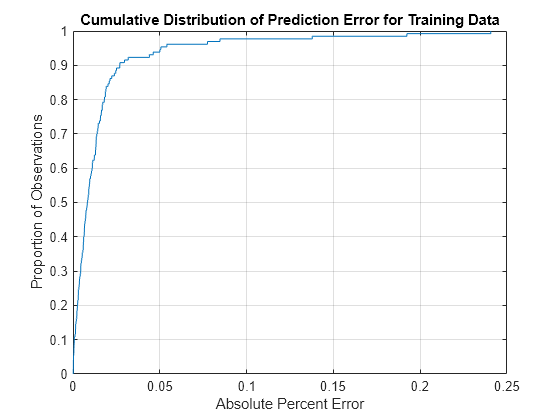
Plot the cumulative distribution of the absolute percent error and compute its summary statistics: minimum, maximum, mean, median, and standard deviation.
figure
[~,apeStatsTrain] = cdfplot(absPercentError)
apeStatsTrain = struct with fields:
       min: 1.1299e-04
       max: 0.2406
      mean: 0.0160
    median: 0.0083
       std: 0.0308
xlabel("Absolute Percent Error")
ylabel("Proportion of Observations")
title("Cumulative Distribution of Prediction Error for Training Data")
Plot Predicted vs. Actual Responses
Visually compare the predicted responses against the actual responses. If the prediction accuracy is perfect, then all the points will lie exactly on a diagonal line of slope 1 and intercept 0. The deviation of an observation point from this "perfect prediction line" is the prediction error for the corresponding observation.
figure
plot(fR_actual,fR_predicted,"o",DisplayName="Observations")
hline = refline(1,0);
hline.DisplayName = "Perfect prediction";

idx = find(absPercentError > 5);
hold on
plot(fR_actual(idx),fR_predicted(idx),"kx",DisplayName="Error > 5%")
hold off

title("Predictions on Training Data")
xlabel("True Response")
ylabel("Predicted Response")
legend(Location="southeast")

Evaluate Trained Model on Test Data Set
To assess the model's degree of generalization and predictive capability, evaluate it with data that it has not seen, specifically the test data kept aside for this purpose. This helps to gauge the model's ability to make accurate predictions on new observations, which is ultimately the goal of training and tuning the model.
Compute Percent Error in Model Predictions
Use the model's predict function on the test data, and compute the prediction error for each observation.
fR_predicted = predict(mdl,dataTest);
fR_actual = dataTest.fR;
percentError = (fR_predicted-fR_actual)./fR_actual*100;
absPercentError = abs(percentError);
resultsTest = addvars(dataTest,fR_predicted,percentError)
resultsTest=30×10 table
           Lp    Wp    ls    ws     ds     h      eR      fR     fR_predicted    percentError
           __    __    __    ___    __    ___    ____    ____    ____________    ____________

    3      40    30    15    7.5     5    1.6    2.33     2.5       2.4286          -2.8542
    7      35    25    25      7     8    1.6    2.33    1.55       1.5753           1.6335
    18     40    30    30     15     5    1.6    2.33     1.3       1.3717           5.5184
    24     45    35    25      5    25    1.6    2.33     1.6       1.6146          0.91085
    39     45    35    30     10    25    1.6    2.33       2       1.9675          -1.6256
    40     50    40    40     20    14    1.6    2.33    1.75        1.792           2.3976
    41     30    20    10      5     3    2.5    2.33    3.25       3.1878          -1.9128
    44     45    35    25      5    20    2.5    2.33     1.5       1.4658           -2.278
    56     30    20    20     10     3    2.5    2.33    2.05       2.0248          -1.2314
    58     40    30    30     15     5    2.5    2.33     1.3       1.3812           6.2499
    59     45    35    30     10    20    2.5    2.33     1.3       1.3857           6.5904
    62     35    25    15      7    10    2.5    2.33    2.25       2.2369         -0.58346
    73     40    30    15     15    10    2.5    2.33     2.1       2.1237           1.1295
    87     35    25    25      7     8    1.6     4.4     1.9       1.9355           1.8674
    98     40    30    30     15     5    1.6     4.4     1.6       1.6424           2.6511
    103    40    30    15    7.5    10    1.6     4.4     1.5       1.5456           3.0414
      ⋮
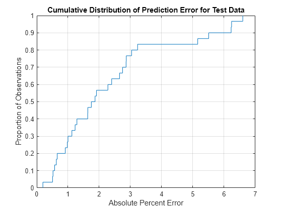
Plot the cumulative distribution of the absolute percent error and compute its summary statistics. Note that most of the predictions have less than 5% absolute error.
figure
[~,apeStatsTest] = cdfplot(absPercentError)
apeStatsTest = struct with fields:
       min: 0.1945
       max: 6.5904
      mean: 2.3415
    median: 1.8085
       std: 1.8569
xlabel("Absolute Percent Error")
ylabel("Proportion of Observations")
title("Cumulative Distribution of Prediction Error for Test Data")
Plot Predicted vs. Actual Responses
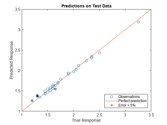
Visually compare the predicted responses against the actual responses. The model performs reasonably well on most of the test data set, but prediction error exceeds 5% for a handful of the observations.
figure
plot(fR_actual,fR_predicted,"o",DisplayName="Observations")
hline = refline(1,0);
hline.DisplayName = "Perfect prediction";

idx = find(absPercentError > 5);
hold on
plot(fR_actual(idx),fR_predicted(idx),"kx",DisplayName="Error > 5%")
hold off

title("Predictions on Test Data")
xlabel("True Response")
ylabel("Predicted Response")
legend(Location="southeast")
Conclusion
In this example, you developed a machine learning model to characterize a custom antenna structure based on its key design parameters. Specifically, you trained a regression model to predict the resonant frequency of a C-shaped microstrip patch antenna on a PCB stack. The trained model performed reasonably well on a test data set not previously seen by the model. However, upon comparison to the excellent prediction accuracy on the training data, it appears that the model did overfit to the training data from which it learned. In summary, this model has good predictive power, but indeed there is room for improvement.
Here are some strategies to improve model generalization and combat overfitting. However, a detailed treatment of this topic is outside the scope of this example.
Perform data augmentation, feature engineering, and/or addtional data preprocessing.
Adjust cross-validation options during training and hyperparameter tuning.
Pursue other DOE methods to procure a data set with a more balanced and continuous distribution.
Helper Functions
The following sections define the local, helper functions used in this example to model the antenna and generate response data using full-wave simulation.
Create Model of C-Shaped Microstrip Patch Antenna
The following local function creates a PCB stack model of the C-shaped microstrip patch antenna. This helper function uses custom, 2D shapes and the pcbStack function, and it includes code to visualize the antenna's structure and parameterization. For all parameter sets in this example, the helper function specifies the ground plane dimensions as 1.15 times the respective outer dimensions of the radiating patch.
function ant = createCShapedPatchAntenna( ...
    Lpmm,Wpmm,lsmm,wsmm,dsmm,hmm,eR,feedparams,options)

arguments
    Lpmm
    Wpmm
    lsmm
    wsmm
    dsmm
    hmm
    eR
    feedparams
    options.Visualize (1,1) logical = false
end

Lp = Lpmm*1e-3;
Wp = Wpmm*1e-3;
ls = lsmm*1e-3;
ws = wsmm*1e-3;
ds = dsmm*1e-3;
h = hmm*1e-3;

GPL = 1.15*Lp;
GPW = 1.15*Wp;

groundplane = antenna.Rectangle( ...
    Length=GPL,Width=GPW,Center=[Lp/2,Wp/2],Name="Ground Plane");
patch = antenna.Rectangle(Length=Lp,Width=Wp,Center=[Lp/2,Wp/2]);
slot = antenna.Rectangle(Length=ls,Width=ws,Center=[Lp-ls/2,Wp-ds-ws/2]);

radiator = patch - slot;
radiator.Name = "Radiator";
substrate = dielectric(Name=sprintf("eR = %g",eR),EpsilonR=eR,Thickness=h);

x0 = feedparams.x0;
y0 = feedparams.y0;
V = feedparams.V;

ant = pcbStack(BoardShape=groundplane,BoardThickness=h, ...
    FeedLocations=[x0,y0,1,3],FeedVoltage=V, ...
    Layers={radiator,substrate,groundplane});

if options.Visualize
    x0mm = x0*1e3;
    y0mm = y0*1e3;

    figure
    show(ant)
    view(3)
    text(Lpmm*34/30,0,0,"h",FontName="FixedWidth")
    text(x0mm-1,y0mm-1,hmm+3,"Feed (x0,y0)", ...
        FontName="FixedWidth",HorizontalAlignment="center")

    figure
    show(ant)
    view(2)
    text(Lpmm/2,0,hmm,"Lp", ...
        FontName="FixedWidth",VerticalAlignment="bottom")
    text(0,Wpmm/2,hmm,"Wp",FontName="FixedWidth")
    text(Lpmm-lsmm/2,Wpmm-dsmm-wsmm,hmm,"ls", ...
        FontName="FixedWidth",VerticalAlignment="bottom")
    text(Lpmm-lsmm,Wpmm-dsmm-wsmm/2,hmm,"ws",FontName="FixedWidth")
    text(Lpmm,Wpmm-dsmm/2,hmm,"ds",FontName="FixedWidth")
end
end
Generate Response Data for Observation
The following local function computes the complex-valued S-parameter and impedance responses using full-wave simulation for a given specification of antenna design parameters.
function [S,Z] = generateObservation(T,feedparams,f,options)

arguments
    T
    feedparams
    f
    options.SaveDataToFile (1,1) logical = true
    options.FileIndex {mustBeInteger,mustBePositive} = 1
    options.FolderName {mustBeTextScalar} = "data"
end

tic
ant = createCShapedPatchAntenna( ...
    T.Lp, T.Wp, ...       % Outer dimensions
    T.ls, T.ws, T.ds, ... % Slot dimensions
    T.h, T.eR, ...        % Substrate parameters
    feedparams);          % Feed parameters
S = sparameters(ant,f);
Z = impedance(ant,f);
tElapsed = toc;
fprintf("%.2f seconds to generate observation %d.\n", ...
    tElapsed,options.FileIndex)

if options.SaveDataToFile
    if ~isfolder(options.FolderName)
        mkdir(options.FolderName)
    end
    filename = fullfile(options.FolderName, ...
        sprintf("%.3d.mat",options.FileIndex));
    save(filename,"T","feedparams","f","S","Z","tElapsed")
end
end
References
[1] S. Bhunia, "Effects of Slot Loading on Microstrip Patch Antennas", International Journal of Wired and Wireless Communications, vol. 1, no. 1, pp. 1-6, Oct. 2012.
[2] U. Özkaya, E. Yiğit, L. Seyfi, Ş. Öztürk, and D. Singh, "Comparative Regression Analysis for Estimating Resonant Frequency of C-Like Patch Antennas", Mathematical Problems in Engineering, vol. 2021, pp. 1-8, Feb. 2021.
[3] E. Yigit, "Operating Frequency Estimation of Slot Antenna by Using Adapted kNN Algorithm", International Journal of Intelligent Systems and Applications in Engineering, vol. 6, no. 1, pp. 29-32, Mar. 2018.
[4] S. Sivaramakrishnan, V. Iyer, T. Gao, and G. Zucchelli, "A Systematic Application of AI Techniques to Antenna Design, Analysis, and Optimization," 2024 54th European Microwave Conference (EuMC), Paris, France, pp. 972-975, Sep. 2024.