Visualize Viewsheds and Coverage Maps Using Terrain
Display viewsheds and coverage maps for an area of interest using satellite imagery and terrain data. A viewshed includes areas that are within line of sight (LOS) of a set of points, and a coverage map includes received power for the areas within range of a set of wireless transmitters. You can use a viewshed as a first-order approximation of a coverage map.
By combining the mapping capabilities in Mapping Toolbox™ with the RF propagation capabilities in Antenna Toolbox™, you can create contoured coverage maps and use the contour data for both visualization and analysis. This example shows you how to:
View imagery and terrain on 2-D maps
View imagery, terrain, and viewsheds on 3-D relief maps
View coverage maps in 2-D using contour plots and bar graphs
Determine whether nearby points are within coverage
View coverage maps for other regions of interest
View Imagery on 2-D Map
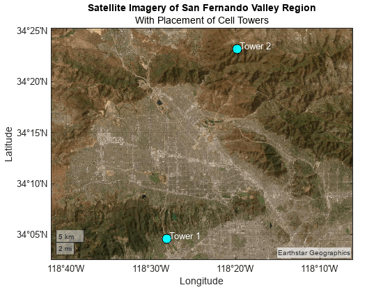
You can view imagery for an area of interest by plotting data into geographic axes. Geographic axes enable you to plot 2-D data over basemaps, explore regions interactively, and add data tips to points of interest.
Specify the geographic coordinates and heights of two cell towers in the San Fernando Valley region. Specify the heights using meters above the terrain.
lat1 = 34.076389;
lon1 = -118.468944;
towerHeight1 = 17.1;
text1 = "Tower 1";

lat2 = 34.386389;
lon2 = -118.329778;
towerHeight2 = 30.5;
text2 = "Tower 2";
Display the locations of the cell towers over a satellite basemap. Throughout the example, create larger maps by increasing the sizes of the figures.
f1 = figure;
fSize = [560 420];
f1.Position(3:4) = fSize;

basemap = "satellite";
geobasemap(basemap)

geoplot([lat1 lat2],[lon1 lon2], ...
    LineStyle="none",Marker="o",MarkerSize=10, ...
    MarkerEdgeColor="k",MarkerFaceColor="c")
Prepare to create a 3-D relief map for the same region by querying the zoom level, latitude limits, and longitude limits of the geographic axes. To ensure that the relief map covers the same region, change the zoom level of the geographic axes to an integer.
gx = gca;
zoomLevel = floor(gx.ZoomLevel);
gx.ZoomLevel = zoomLevel;

[latlim,lonlim] = geolimits(gx);
Customize the map by labeling the cell towers and adding a title.
txtDelta = 0.005;
text(lat1 + txtDelta,lon1 + txtDelta,text1,Color="w")
text(lat2 + txtDelta,lon2 + txtDelta,text2,Color="w")
title("Satellite Imagery of San Fernando Valley Region")
subtitle("With Placement of Cell Towers")
View Terrain on 2-D Map
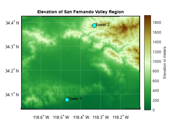
Visualize the terrain for the same area of interest by plotting imported elevation data into an axesm-based map. axesm-based maps enable you to display geographic data using a map projection.
Read Terrain Elevation Data
Read terrain elevation data for the area of interest from a Web Map Service (WMS) server. WMS servers provide geospatial data such as elevation, temperature, and weather from web-based sources.
Search the WMS Database for terrain elevation data hosted by MathWorks®. The wmsfind function returns search results as layer objects. A layer is a data set that contains a specific type of geographic information, in this case elevation data.
layer = wmsfind("mathworks",SearchField="serverurl");
layer = refine(layer,"elevation");
Read the elevation data from the layer into the workspace as an array and a spatial reference object in geographic coordinates. Get quantitative data by specifying the image format as BIL.
[Z,RZ] = wmsread(layer,Latlim=latlim,Lonlim=lonlim,ImageFormat="image/bil");Prepare the elevation data for plotting by converting the data type to double.
Z = double(Z);
Find Tower Elevations
Calculate the terrain elevation at the base of each cell tower. The elevations are in meters above mean sea level.
height1 = geointerp(Z,RZ,lat1,lon1,"nearest")height1 = 177
height2 = geointerp(Z,RZ,lat2,lon2,"nearest")height2 = 1422
Visualize Elevation and Tower Locations
Create an axesm-based map with an appropriate projection for the region. Then, display the elevation data as a surface using an appropriate colormap. Note that the areas of highest elevation are in the northeast corner.
f2 = figure;
f2.Position(3:4) = fSize;

usamap(Z,RZ)
geoshow(Z,RZ,DisplayType="texturemap")
demcmap(Z,256)

geoshow(lat1,lon1,DisplayType="point",ZData=height1, ...
    MarkerEdgeColor="k",MarkerFaceColor="c",MarkerSize=10,Marker="o")
geoshow(lat2,lon2,DisplayType="point",ZData=height2, ...
     MarkerEdgeColor="k",MarkerFaceColor="c",MarkerSize=10,Marker="o")

textm(lat1 + txtDelta,lon1 + txtDelta,text1)
textm(lat2 + txtDelta,lon2 + txtDelta,text2)
title("Elevation of San Fernando Valley Region")

cb = colorbar;
cb.Label.String = "Elevation in meters";
View Imagery, Terrain, and Viewshed on 3-D Relief Map
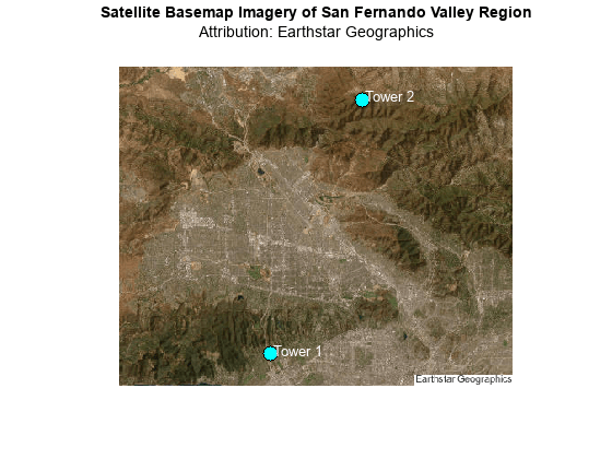
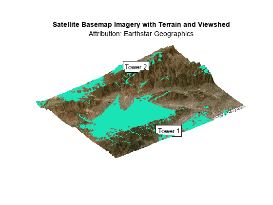
Visualize the imagery, terrain, and viewshed for the region by plotting the terrain data over a basemap image in a standard axes. Basemap images enable you to provide geographic context for plot types that geographic axes do not support, such as 3-D surfaces.
Read Basemap Image
Read a basemap image using the same basemap, geographic limits, and zoom level as the geographic axes. The readBasemapImage function reads the image into the workspace as an array, a spatial reference object in Web Mercator (WGS 84/Pseudo-Mercator) coordinates, and an attribution string.
[A,RA,attrib] = readBasemapImage(basemap,latlim,lonlim,zoomLevel);
To display the cell tower locations over the basemap image, you must first project the geographic coordinates to Web Mercator coordinates.
proj = RA.ProjectedCRS;
[x1,y1] = projfwd(proj,lat1,lon1);
[x2,y2] = projfwd(proj,lat2,lon2);
Plot the projected coordinates over the basemap image. Note that this visualization is similar to the geographic axes visualization.
f3 = figure;
f3.Position(3:4) = fSize;

axis off
hold on

mapshow(A,RA)
plot([x1 x2],[y1 y2], ...
    LineStyle="none",Marker="o",MarkerSize=10, ...
    MarkerEdgeColor="k",MarkerFaceColor="c")

txtDeltaXY = 500;
text(x1 + txtDeltaXY,y1 + txtDeltaXY,text1,Color="w")
text(x2 + txtDeltaXY,y2 + txtDeltaXY,text2,Color="w")
title("Satellite Basemap Imagery of San Fernando Valley Region")
subtitle("Attribution: " + attrib)
Calculate Viewsheds from Towers
Read the terrain data again, this time using array dimensions and geographic limits that match the dimensions and limits of the basemap image.
[latlim,lonlim] = projinv(proj,RA.XWorldLimits,RA.YWorldLimits);
szA = RA.RasterSize;

[Z,RZ] = wmsread(layer,Latlim=latlim,Lonlim=lonlim, ...
    ImageHeight=szA(1),ImageWidth=szA(2),ImageFormat="image/bil");
Z = double(Z);
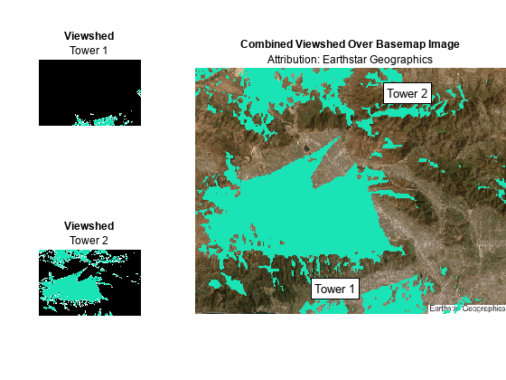
Calculate the viewshed for each tower by specifying the terrain data and the cell tower coordinates. The first argument returned by each viewshed call indicates visible areas using 1 values and obscured areas using 0 values.
[vis1,visR1] = viewshed(Z,RZ,lat1,lon1,towerHeight1);
[vis2,visR2] = viewshed(Z,RZ,lat2,lon2,towerHeight2);
Calculate the combined viewshed for both towers. To avoid plotting the obscured areas, replace the 0 values with NaN values.
visCombined = vis1 | vis2;
vis = visCombined;
vis = double(vis);
vis(vis == 0) = NaN;
visR = visR2;
Extract the geographic coordinates of the elevation data from its spatial reference object. Then, project the coordinates to Web Mercator coordinates.
[latz,lonz] = geographicGrid(RZ);
[xz,yz] = projfwd(proj,latz,lonz);
View Individual and Combined Viewsheds
Display the viewshed for each tower and the combined viewshed for both towers in a tiled layout.
Define a colormap for the viewshed. Use turquoise for visible areas and black for obscured areas.
cmapt = [0 0 0];
covcolor = [0.1034  0.8960  0.7150];
cmapt(2,:,:) = covcolor;
Create a tiled layout. Display the viewshed for the individual towers on the left.
f4 = figure;
f4.Position(3:4) = fSize;

clim([0 1])
colormap(cmapt)
tiledlayout(2,3,Padding="tight",TileSpacing="tight")

nexttile
geoshow(vis1,visR1,EdgeColor="none",DisplayType="surface")
axis off
title("Viewshed")
subtitle("Tower 1")

nexttile(4)
geoshow(vis2,visR2,EdgeColor="none",DisplayType="surface")
axis off
title("Viewshed")
subtitle("Tower 2")
Display the basemap image and the combined viewshed on the right. Specify the z-coordinates for the labels using the terrain height (above mean sea level) and the tower height (above the terrain).
nexttile([2,2])
mapshow(A,RA)
hold on
mapshow(xz,yz,vis,EdgeColor="none",DisplayType="surface")
axis off

zdelta = 150;
z1 = height1 + towerHeight1 + zdelta;
z2 = height2 + towerHeight2 + zdelta;

text(x1,y1,z1,text1,Color="k",EdgeColor="k",BackgroundColor="w")
text(x2,y2,z2,text2,Color="k",EdgeColor="k",BackgroundColor="w")
title("Combined Viewshed Over Basemap Image")
subtitle("Attribution: " + attrib)
View Basemap Image and Viewshed on 3-D Relief Map
Prepare the combined viewshed for plotting.
Find the indices of visible areas in the combined viewshed.
Replace the visible areas in the combined viewshed with the terrain data (the corresponding values of
Z).
[row,col] = find(visCombined);
sz = size(visCombined);
ind = sub2ind(sz,row,col);
vis(ind) = Z(ind);
Create a new figure that uses the same colormap as the tiled layout. Remove the axes lines and enable the plot to extend to the edges of the axes.
f5 = figure;
f5.Position(3:4) = fSize;

colormap(covcolor)

hold on
axis off
axis tight
Visualize the basemap image, viewshed, and terrain using surfaces.
Display the terrain by draping the basemap image over the elevation data. Specify the z-coordinates using the terrain data, and specify the surface colors using the image data.
Display the combined viewshed.
Customize the plot by adding text labels and a title.
View the plot in 3-D. Adjust the data aspect ratio so that elevation scale is comparable to the xy-scale.
mapshow(xz,yz,Z,DisplayType="surface",CData=A)

mapshow(xz,yz,vis,EdgeColor="none",DisplayType="surface")

text(x1,y1,z1,text1,Color="k",EdgeColor="k",BackgroundColor="w")
text(x2,y2,z2,text2,Color="k",EdgeColor="k",BackgroundColor="w")
title("Satellite Basemap Imagery with Terrain and Viewshed")
subtitle("Attribution: " + attrib)

daspect([1 1 0.25])
view(3)
Visualize Coverage Maps in 2-D
A viewshed is comparable to a wireless coverage map that includes only line-of-sight (LOS) propagation. You can create more detailed coverage maps and calculate received power by using transmitter antenna sites and propagation models.
Calculate Coverage Map
Create a transmitter site for each cell tower. Then, calculate the coverage map and return the result as a propagationData object. By default, the coverage function uses a Longley-Rice propagation model and incorporates diffraction over terrain.
txTower1 = txsite(Name=text1,Latitude=lat1,Longitude=lon1);
txTower2 = txsite(Name=text2,Latitude=lat2,Longitude=lon2);
txsites = [txTower1; txTower2];
pd = coverage(txsites);
Extract latitude and longitude values, power values, and power levels from the propagationData object by using the propagationDataGrid helper function.
dataVariableName = "Power";
maxrange = [30000 30000];
[lats,lons,data,levels] = propagationDataGrid(pd,dataVariableName,maxrange,txsites);
Find the limits of the quadrangle that bounds the coverage map.
covaoi = aoiquad(lats,lons);
[covlatlim,covlonlim] = bounds(covaoi);
Define a colormap using the power levels. Create a new figure that uses the power levels colormap.
cmap = turbo(length(levels));
climLevels = [min(levels) max(levels)+10];

f6 = figure;
f6.Position(3:4) = fSize;

colormap(cmap)
clim(climLevels)
hold on
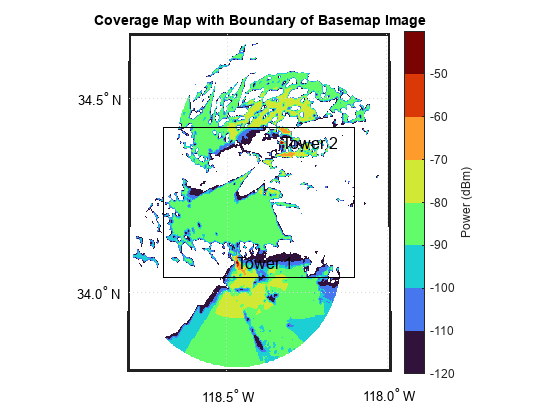
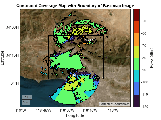
Create an axesm-based map with an appropriate projection for the region. Display the coverage map, a rectangle that represents the San Fernando Valley region, and the transmitter sites on the map. Note that the coverage map extends beyond the San Fernando Valley region.
usamap(covlatlim,covlonlim)
geoshow(lats,lons,data,DisplayType="surface")
geoshow(latlim([1 2 2 1 1]),lonlim([1,1,2,2,1]),Color="k")

textm(lat1,lon1,text1,Color="k",FontSize=12)
textm(lat2,lon2,text2,Color="k",FontSize=12)
title("Coverage Map with Boundary of Basemap Image")

cb = colorbar;
cb.Label.String = "Power (dBm)";
cb.Ticks = levels;
View Contoured Coverage Map on Basemap Image
Project the geographic coordinates of the coverage map to Web Mercator coordinates.
[cx,cy] = projfwd(proj,lats,lons);
Create a figure that uses the power levels colormap.
f7 = figure;
f7.Position(3:4) = fSize;

colormap(cmap)
clim(climLevels)
axis off
hold on
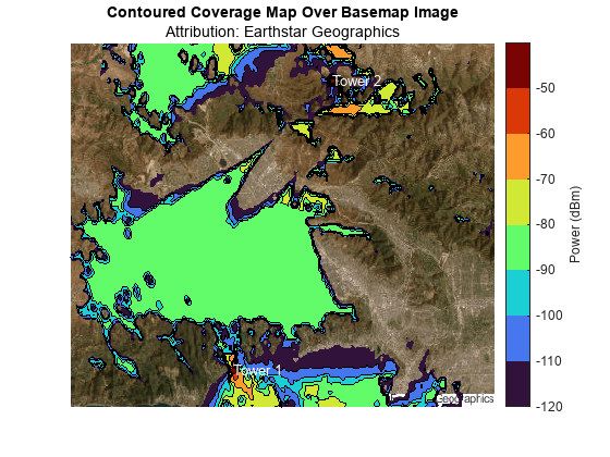
Contour the coverage map, specifying the contour levels as the power levels, and display the result over the basemap image. Change the limits of the map to match the San Fernando Valley region.
mapshow(A,RA)
contourf(cx,cy,data,LevelList=levels)

xlim(RA.XWorldLimits)
ylim(RA.YWorldLimits)

text(x1,y1,text1,Color="w")
text(x2,y2,text2,Color="w")
title("Contoured Coverage Map Over Basemap Image")
subtitle("Attribution: " + attrib)

cb = colorbar;
cb.Label.String = "Power (dBm)";
cb.Ticks = levels;
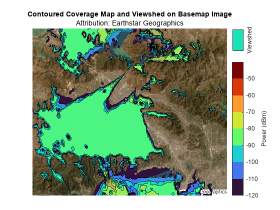
View Contoured Coverage Map and Viewshed on Basemap Image
Project the geographic coordinates of the combined viewshed to Web Mercator coordinates.
[vlat,vlon] = geographicGrid(visR);
[vx,vy] = projfwd(proj,vlat,vlon);
Display the coverage map and viewshed over the basemap image by using contour plots. You can create a map with two colorbars by overlaying two axes objects.
Use the first axes to display the basemap image, the coverage map, and a colorbar for the coverage map.
f8 = figure;
f8.Position(3:4) = fSize;

ax1 = axes;
hold(ax1,"on")
axis(ax1,"off")
clim(ax1,climLevels)
colormap(ax1,cmap)

mapshow(ax1,A,RA)
contourf(ax1,cx,cy,data,LevelList=levels);

xlim(ax1,RA.XWorldLimits)
ylim(ax1,RA.YWorldLimits)
title(ax1,"Contoured Coverage Map and Viewshed on Basemap Image")
subtitle("Attribution: " + attrib)

cb1 = colorbar(ax1);
cb1.Label.String = "Power (dBm)";
cb1.Ticks = levels;
Use the second axes to display the viewshed and a colorbar for the viewshed.
ax2 = axes(Visible="off");
hold(ax2,"on")
colormap(ax2,covcolor)

[~,visContourMap] = contourf(ax2,vx,vy,vis,LevelList=0.5:1:1.5);

cb2 = colorbar(ax2);
cb2.Label.String = "Viewshed";
cb2.Ticks = [];
Reposition the axes objects and the colorbars.
ax1.Position = [ax1.Position(1) ax1.Position(2)-0.04 ax1.Position(3) ax1.Position(4)];
ax2.Position = ax1.Position;
cb1.Position = [cb1.Position(1) cb1.Position(2) cb1.Position(3) cb1.Position(4)*0.8];
cb2.Position = [cb2.Position(1) 0.76 cb2.Position(3) 0.1];
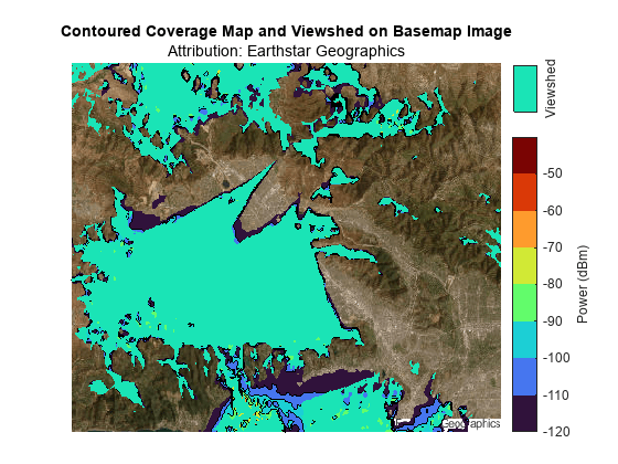
In addition to LOS analysis, the coverage map incorporates diffraction over terrain. As a result, the coverage map extends beyond the viewshed.
Adjust the transparency of the viewshed. When you decrease the value of faceAlpha, the viewshed becomes more transparent and you can see the coverage map beneath.
faceAlpha = 0.3;
visContourMap.FaceAlpha = faceAlpha;
View Contoured Coverage Map on Geographic Axes
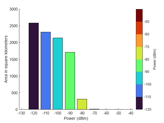
To display a contoured coverage map over geographic axes, contour the coverage map using the contourDataGrid helper function. Each row of the returned geospatial table corresponds to a power level and includes the contour shape, the area of the contour shape in square kilometers, the minimum power for the level, and the power range for the level. The area value for each contour shape includes the regions that are covered by other contour shapes.
GT = contourDataGrid(lats,lons,data,levels);
disp(GT)
       Shape        Area (sq km)    Perimeter (km)    Power (dBm)    Power Range (dBm)
    ____________    ____________    ______________    ___________    _________________

    geopolyshape       2588.9         1.5139e+06         -120          -120    -110
    geopolyshape         2314         1.5045e+06         -110          -110    -100
    geopolyshape       2134.4         1.5159e+06         -100          -100     -90
    geopolyshape       1712.9         1.4211e+06          -90           -90     -80
    geopolyshape       309.79         5.0189e+05          -80           -80     -70
    geopolyshape       13.563              45401          -70           -70     -60
    geopolyshape       1.8949             9214.1          -60           -60     -50
    geopolyshape      0.67629             4408.2          -50           -50     -40
Plot the contoured coverage map and a rectangle that represents the San Fernando Valley region into geographic axes.
f9 = figure;
f9.Position(3:4) = fSize;

geobasemap satellite
colormap(cmap)
clim(climLevels)
hold on

hp = geoplot(GT,ColorVariable="Power (dBm)",EdgeColor="k",FaceAlpha=1);
boundary = geoplot(latlim([1 2 2 1 1]),lonlim([1,1,2,2,1]),Color="k",LineWidth=2);

text(lat1,lon1,text1,Color="w")
text(lat2,lon2,text2,Color="w")
title("Contoured Coverage Map with Boundary of Basemap Image")

cb = colorbar;
cb.Label.String = "Power (dBm)";
cb.Ticks = levels;
Zoom the map into the San Fernando Valley region and delete the boundary.
geolimits(latlim,lonlim)
delete(boundary)
title("Contoured Coverage Map at Boundary of Basemap Image")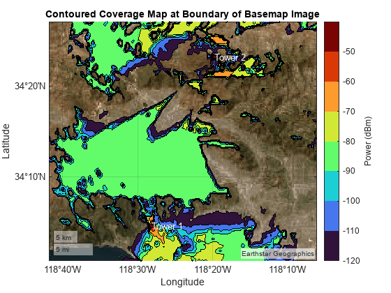
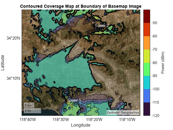
Adjust the transparency of the coverage map. When you decrease the value of faceAlpha, the coverage map becomes more transparent and you can see the basemap beneath.
faceAlpha = 0.3;
hp.FaceAlpha = faceAlpha;
View Bar Graph of Coverage Area
Create a bar graph that shows the coverage area in square kilometers for each power level. As the power level increases, the coverage area decreases.
figure
colormap(cmap)
clim(climLevels)
hold on

bar(GT.("Power (dBm)"),GT.("Area (sq km)"),FaceColor="flat",CData=cmap);
ylabel("Area in square kilometers")
xlabel("Power (dBm)")

cb = colorbar;
cb.Label.String = "Power (dBm)";
cb.Ticks = levels;
Determine If Points Are Within Coverage
Determine whether points within the San Fernando Valley region are within coverage.
Calculate Coverage at Point Locations
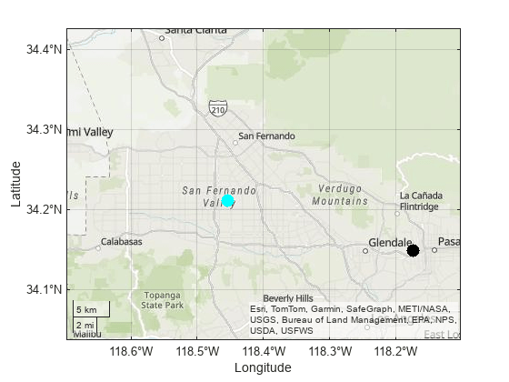
Specify the locations of two points near the cell towers. Determine whether the points are within coverage by using the incoverage helper function. The result indicates the first point is in coverage and the second point is not in coverage.
locationLats = [34.2107 34.1493];
locationLons = [-118.4545 -118.1744];

[tf,powerLevels] = incoverage(locationLats,locationLons,GT);
disp(tf)
   1
   0
Display the power levels. The result -Inf indicates that the second point is not in coverage.
disp(powerLevels)
   -90
  -Inf
Display the point that is in coverage using a cyan marker and the point that is not in coverage using a black marker.
f10 = figure;
f10.Position(3:4) = fSize;

geobasemap topographic
hold on
geotickformat dd
geolimits(latlim,lonlim)

geoplot(locationLats(tf),locationLons(tf),"o", ...
    MarkerEdgeColor="c",MarkerFaceColor="c",MarkerSize=10)
geoplot(locationLats(~tf),locationLons(~tf),"o", ...
    MarkerEdgeColor="k",MarkerFaceColor="k",MarkerSize=10)
Interactively Select Points and Calculate Coverage at Point Locations
Select points and determine whether they are in coverage.
Set up a map that uses the power levels colormap. Then, plot the contoured coverage map.
f11 = figure;
f11.Position(3:4) = fSize;

geobasemap topographic
geolimits(latlim,lonlim)
hold on
geotickformat dd
colormap(cmap)
clim(climLevels)

contourPlot = geoplot(GT,ColorVariable="Power (dBm)",EdgeColor="k",FaceAlpha=1);

cb = colorbar;
cb.Label.String = "Power (dBm)";
cb.Ticks = levels(1:end);
Select the points. Use predefined points by specifying interactivelySelectPoints as false. Alternatively, you can interactively select points by specifying interactivelySelectPoints as true. Specify the number of points to interactively select by specifying a value for numberOfPoints.
interactivelySelectPoints =false;
if interactivelySelectPoints
    numberOfPoints = 4; %#ok<*UNRCH>
    title("Select " + string(numberOfPoints) + " Points")
    pts = ginput(numberOfPoints);
else
    pts = [ ...
        34.0732 -118.4652
        34.1880 -118.2000
        34.2200 -118.6172
        34.3849 -118.5472];
end
Determine whether each point is within coverage. If the point is not within coverage, display it on the map in black. If the point is within coverage, display it on the map using the color associated with its power level.
for k = 1:size(pts,1)
    latpoint = pts(k,1);
    lonpoint = pts(k,2);
    [tf,powerLevel] = incoverage(latpoint,lonpoint,GT);

    if ~tf
        color = [0 0 0];
    else
        index = GT.("Power (dBm)") == powerLevel;
        color = cmap(index,:,:);
    end

    h = geoplot(latpoint,lonpoint,"o",MarkerEdgeColor=color, ...
        MarkerFaceColor=color,MarkerSize=10);
    dt = datatip(h);
    dtrow = dataTipTextRow("Power",powerLevel);
    h.DataTipTemplate.DataTipRows(end+1) = dtrow;
end
title("Selected Points")
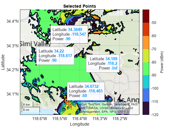
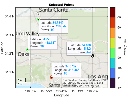
Toggle off the contour plot by setting showContourPlot to false. The color of each point indicates its power level.
showContourPlot = false;
contourPlot.Visible = showContourPlot;
Create Geographic Coverage Maps for Other Regions
The geocoverage helper function calculates or displays a coverage map for the specified transmitter sites. When you specify an output argument, the function returns a geospatial table.
T = geocoverage(txsites);
disp(T)
       Shape        Area (sq km)    Perimeter (km)    Power (dBm)    Power Range (dBm)
    ____________    ____________    ______________    ___________    _________________

    geopolyshape       2588.9         1.5139e+06         -120          -120    -110
    geopolyshape         2314         1.5045e+06         -110          -110    -100
    geopolyshape       2134.4         1.5159e+06         -100          -100     -90
    geopolyshape       1712.9         1.4211e+06          -90           -90     -80
    geopolyshape       309.79         5.0189e+05          -80           -80     -70
    geopolyshape       13.563              45401          -70           -70     -60
    geopolyshape       1.8949             9214.1          -60           -60     -50
    geopolyshape      0.67629             4408.2          -50           -50     -40
When you omit the output argument, the function contours the coverage map and displays the result over a basemap.
basemap = "topographic";
geocoverage(txsites(1),basemap)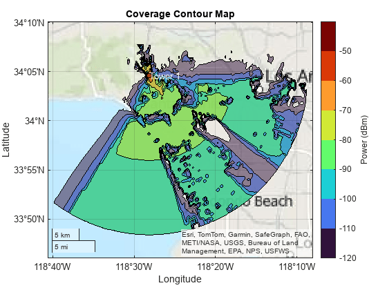
You can use the geocoverage helper function to create coverage maps for other locations. For example, create a coverage map for cell towers near Boston. The geocoverage function calculates coverage data for up to 30 kilometers from the transmitter sites.
names = ["Clarendon St.","Cambridge St.","Albany St."];
bostonLat = [42.348722 42.361222 42.338444];
bostonLon = [-71.075889 -71.069778 -71.065611];
bostonH = [260 30 23];
freq = [852.637e6 862.012e6 862.012e6];
txs = txsite(Name=names,Latitude=bostonLat,Longitude=bostonLon, ...
             AntennaHeight=bostonH,TransmitterFrequency=freq);
geocoverage(txs,basemap)
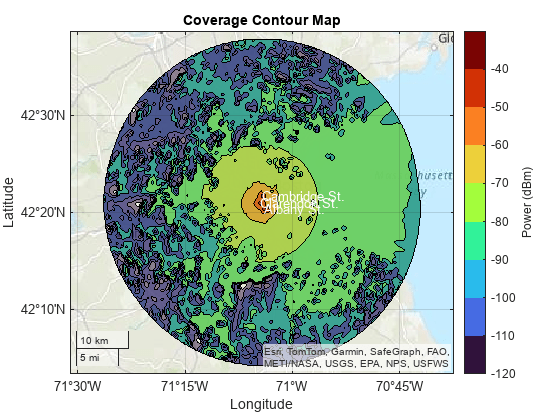
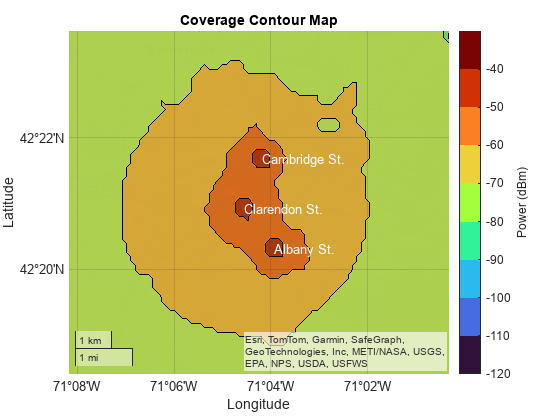
The cell towers are close together. View the area immediately around the towers by zooming in on the coverage map.
gx = gca;
gx.ZoomLevel = 12;
Helper Functions
The propagationDataGrid helper function extracts the latitude and longitude values clats and clons, the power values cdata, and the power levels levels from the propagation data object pd with data variable dataVariableName, using the transmitter sites txsites and the maximum range in meters from the transmitter sites maxrange. Within the function:
Create regularly spaced grids of latitude and longitude values from the propagation data object.
Determine which latitude and longitude values are within range of the transmitter sites.
Create a grid of power values by interpolating the propagation data. Interpolate only the values that are within range of the transmitter sites.
Determine the power levels by discretizing the data grid.
function [clats,clons,cdata,levels] = propagationDataGrid(pd,dataVariableName,maxrange,txsites)
% Extract propagation data grid from propagationData object

    % Create grids of latitude and longitude values
    imageSize = [512 512];
    lats = pd.Data.Latitude;
    lons = pd.Data.Longitude;
    data = pd.Data.(dataVariableName);

    [lonmin,lonmax] = bounds(lons);
    [latmin,latmax] = bounds(lats);
    lonsv = linspace(lonmin,lonmax,imageSize(2));
    latsv = linspace(latmin,latmax,imageSize(1));
    [clons,clats] = meshgrid(lonsv,latsv);

    % Determine which latitude and longitude values are within range of the
    % transmitters
    txlat = [txsites.Latitude]';
    txlon = [txsites.Longitude]';

    numTx = size(txlat,1);
    gc = nan(numel(clons),numTx);
    for txInd = 1:numTx
        gc(:,txInd) = distance(txlat(txInd),txlon(txInd),clats(:),clons(:),wgs84Ellipsoid);
    end
    isInRange = any(gc <= maxrange,2);

    % Create grid of power values
    cdata = nan(imageSize);
    cdata(isInRange) = interp(pd,clats(isInRange),clons(isInRange), ...
        DataVariableName=dataVariableName);

    % Determine power levels
    [bmin,bmax] = bounds(data);
    levels = max(bmin,-120):10:bmax;
    datalevels = sort(levels);
    % Need max bin edge to include all values
    maxBin = max(max(datalevels(:)),max(cdata(:))) + 1;
    bins = [datalevels(:); maxBin];
    cdata = discretize(cdata,bins,datalevels);
end
The contourDataGrid helper function contours a data grid created using the propagationDataGrid helper function and returns the result as a geospatial table. Each row of the table corresponds to a power level and includes the contour shape, the area of the contour shape in square kilometers, the minimum power for the level, and the power range for the level. Within the function:
Ensure that the function contours power values below the minimum power level by replacing
NaNvalues in the power grid with a large negative number.Prepare to contour the data by projecting the latitude and longitude coordinates to xy-coordinates. Contouring xy-coordinates is more performant than contouring latitude and longitude coordinates.
Contour the projected coordinates using the
contourffunction. Specify the contour levels as the power levels. Thecontourffunction returns a matrix that contains, for each power level, the coordinates of the contour lines.Prepare to process the data for each contour line by initializing several variables.
Process the data for each contour line. Remove contour lines made of collinear points or fewer than three points. Unproject the coordinates.
Create contour shapes from the unprojected coordinates. Include the contour shapes, the areas of the shapes, the perimeters of the shapes, and the power levels in a geospatial table.
Condense the geospatial table into a new geospatial table with one row per power level. Each row contains one combined contour shape (that includes all contour shapes for the power level), the total area of the combined contour shape, the total perimeter of the combined contour shape, the minimum power for the level, and the power range for the level.
Clean up the geospatial table. Convert the area of each shape to square kilometers, ensure that small contours appear on top of large contours by sorting the rows, and rename the table variables.
function GT = contourDataGrid(latd,lond,data,levels)
% Contour data grid created from propagationDataGrid helper function

    % Replace NaN values in power grid with a large negative number
    data(isnan(data)) = min(levels) - 1000;

    % Project the coordinates using an equal-area projection
    proj = projcrs(102008,"Authority","ESRI");
    [xd,yd] = projfwd(proj,latd,lond);

    % Contour the projected data
    fig = figure("Visible","off");
    obj = onCleanup(@()close(fig));
    c = contourf(xd,yd,data,LevelList=levels);

    % Initialize variables
    x = c(1,:);
    y = c(2,:);
    n = length(y);
    k = 1;
    index = 1;
    levels = zeros(n,1);
    latc = cell(n,1);
    lonc = cell(n,1);

    % Process the coordinates of the projected contours
    while k < n
        level = x(k);
        numVertices = y(k);
        yk = y(k+1:k+numVertices);
        xk = x(k+1:k+numVertices);
        k = k + numVertices + 1;

        [first,last] = findNanDelimitedParts(xk);
        jindex = 0;
        jy = {};
        jx = {};

        for j = 1:numel(first)
            % Process the j-th part of the k-th level
            s = first(j);
            e = last(j);
            cx = xk(s:e);
            cy = yk(s:e);
            if cx(end) ~= cx(1) && cy(end) ~= cy(1)
                cy(end+1) = cy(1); %#ok<*AGROW>
                cx(end+1) = cx(1);
            end

            if j == 1 && ~ispolycw(cx,cy)
                % First region must always be clockwise
                [cx,cy] = poly2cw(cx,cy);
            end

            % Filter regions made of collinear points or fewer than 3 points
            if ~(length(cx) < 4 || all(diff(cx) == 0) || all(diff(cy) == 0))
                jindex = jindex + 1;
                jy{jindex,1} = cy(:)';
                jx{jindex,1} = cx(:)';
            end

        end

        % Unproject the coordinates of the processed contours
        [jx,jy] = polyjoin(jx,jy);
        if length(jy) > 2 && length(jx) > 2
            [jlat,jlon] = projinv(proj,jx,jy);
            latc{index,1} = jlat(:)';
            lonc{index,1} = jlon(:)';
            levels(index,1) = level;
            index = index + 1;
        end
    end

    % Create contour shapes from the unprojected coordinates. Include the
    % contour shapes, the areas of the shapes, the perimeters of the
    % shapes, and the power levels in a geospatial table.
    latc = latc(1:index-1);
    lonc = lonc(1:index-1);
    Shape = geopolyshape(latc,lonc);

    Area = area(Shape);

    Perimeter = perimeter(Shape);

    levels = levels(1:index-1);
    Levels = levels;

    allPartsGT = table(Shape,Area,Perimeter,Levels);

    % Condense the geospatial table into a new geospatial table with one
    % row per power level.
    GT = table.empty;
    levels = unique(allPartsGT.Levels);
    for k = 1:length(levels)
        gtLevel = allPartsGT(allPartsGT.Levels == levels(k),:);
        tLevel = geotable2table(gtLevel,["Latitude","Longitude"]);
        [lon,lat] = polyjoin(tLevel.Longitude,tLevel.Latitude);
        Shape = geopolyshape(lat,lon);
        Levels = levels(k);
        Area = area(Shape);
        Perimeter = perimeter(Shape);
        GT(end+1,:) = table(Shape,Area,Perimeter,Levels);
    end

    maxLevelDiff = max(abs(diff(GT.Levels)));
    LevelRange = [GT.Levels GT.Levels + maxLevelDiff];
    GT.LevelRange = LevelRange;

    % Clean up the geospatial table
    GT.Area = GT.Area/1e6;
    GT = sortrows(GT,"Area","descend");
    GT.Properties.VariableNames = ...
        ["Shape","Area (sq km)","Perimeter (km)","Power (dBm)","Power Range (dBm)"];
end
The incoverage helper function determines whether the points with latitude values lat and longitude values lon are within the coverage map defined by the geospatial table T. Within the function:
Determine whether the points are within the coverage map and return the results in
in. The elements ofinare1(true) when the corresponding points are within coverage.Determine the power levels for the points and return the results in
powerLevels. A value of-Infindicates that the corresponding point is not within coverage.
function [in,powerLevels] = incoverage(lat,lon,T)
% Query points in coverage

    % Determine whether points are within coverage
    tf = false(length(T.Shape),length(lat));
    for k = 1:length(T.Shape)
        tf(k,:) = isinterior(T.Shape(k),geopointshape(lat,lon));
    end

    % Determine the power levels for the points
    in = false(length(lat),1);
    powerLevels = -inf(length(lat),1);
    for k = 1:length(in)
        v = tf(:,k);
        in(k) = any(v);
        if in(k)
            powerLevels(k) = max(T{v,"Power (dBm)"});
        end
    end
end
The geocoverage helper function calculates or displays a coverage map for the transmitter sites txsites. Within the function:
Calculate the coverage map by using the
coveragefunction. Then, contour the coverage map by using theprogagationDataGridandcontourDataGridhelper functions.When you do not specify an output argument, the function displays the contoured coverage map over geographic axes using the basemap
basemap.When you do specify an output argument, the function returns the result as a geospatial table.
function varargout = geocoverage(txsites,basemap)
% Display or calculate contoured coverage map

    % Calculate and contour the coverage map
    pd = coverage(txsites);
    dataVariableName = "Power";
    maxrange = 30000*ones(1,length(txsites));
    [lats,lons,data,levels] = propagationDataGrid(pd,dataVariableName,maxrange,txsites);
    GT = contourDataGrid(lats,lons,data,levels);

    % If you do not specify an output argument, display the coverage map
    if nargout == 0
        if nargin < 2
            basemap = "satellite";
        end

        cmap = turbo(length(levels));
        fig = figure;
        fig.Position(3:4) = [560 420];

        geobasemap(basemap)

        geoplot(GT,ColorVariable="Power (dBm)",EdgeColor="k",FaceAlpha=0.5)
        colormap(cmap)
        clim([min(levels) max(levels)+10])

        h = colorbar;
        h.Label.String = "Power (dBm)";
        h.Ticks = levels;

        for k = 1:length(txsites)
            latt = txsites(k).Latitude;
            lont = txsites(k).Longitude;
            text(latt,lont,txsites(k).Name,Color="w")
        end

        title("Coverage Contour Map")
    % If you specify an output argument, return a geospatial table
    else
        varargout{1} = GT;
    end
end
The findNanDelimitedParts helper function finds the indices of the first and last elements of each NaN-separated part of the array x. The contourDataGrid helper function uses findNanDelimitedParts.
function [first,last] = findNanDelimitedParts(x)
% Find indices of the first and last elements of each part in x.
% x can contain runs of multiple NaNs, and x can start or end with
% one or more NaNs.

    n = isnan(x(:));

    firstOrPrecededByNaN = [true; n(1:end-1)];
    first = find(~n & firstOrPrecededByNaN);

    lastOrFollowedByNaN = [n(2:end); true];
    last = find(~n & lastOrFollowedByNaN);
end
See Also
Functions
viewshed(Mapping Toolbox) |contourf|coverage|geoplot(Mapping Toolbox) |readBasemapImage(Mapping Toolbox)