crepePreprocess
Syntax
Description
Examples
Download CREPE Network
Download and unzip the Audio Toolbox™ model for CREPE.
Type crepe
at the Command Window. If the Audio Toolbox model for CREPE is not installed, then the function provides a link to the location of the network weights. To download the model, click the link and unzip the file to a location on the MATLAB path.
Alternatively, execute these commands to download and unzip the CREPE model to your temporary directory.
downloadFolder = fullfile(tempdir,'crepeDownload'); loc = websave(downloadFolder,'https://ssd.mathworks.com/supportfiles/audio/crepe.zip'); crepeLocation = tempdir; unzip(loc,crepeLocation) addpath(fullfile(crepeLocation,'crepe'))
Check that the installation is successful by typing crepe
at the Command Window. If the network is installed, then the function returns a DAGNetwork
(Deep Learning Toolbox) object.
crepe
ans = DAGNetwork with properties: Layers: [34×1 nnet.cnn.layer.Layer] Connections: [33×2 table] InputNames: {'input'} OutputNames: {'pitch'}
Load Pretrained CREPE Network
Load a pretrained CREPE convolutional neural network and examine the layers and classes.
Use crepe
to load the pretrained CREPE network. The output net
is a DAGNetwork
(Deep Learning Toolbox) object.
net = crepe
net = DAGNetwork with properties: Layers: [34×1 nnet.cnn.layer.Layer] Connections: [33×2 table] InputNames: {'input'} OutputNames: {'pitch'}
View the network architecture using the Layers
property. The network has 34 layers. There are 13 layers with learnable weights, of which six are convolutional layers, six are batch normalization layers, and one is a fully connected layer.
net.Layers
ans = 34×1 Layer array with layers: 1 'input' Image Input 1024×1×1 images 2 'conv1' Convolution 1024 512×1×1 convolutions with stride [4 1] and padding 'same' 3 'conv1_relu' ReLU ReLU 4 'conv1-BN' Batch Normalization Batch normalization with 1024 channels 5 'conv1-maxpool' Max Pooling 2×1 max pooling with stride [2 1] and padding [0 0 0 0] 6 'conv1-dropout' Dropout 25% dropout 7 'conv2' Convolution 128 64×1×1024 convolutions with stride [1 1] and padding 'same' 8 'conv2_relu' ReLU ReLU 9 'conv2-BN' Batch Normalization Batch normalization with 128 channels 10 'conv2-maxpool' Max Pooling 2×1 max pooling with stride [2 1] and padding [0 0 0 0] 11 'conv2-dropout' Dropout 25% dropout 12 'conv3' Convolution 128 64×1×128 convolutions with stride [1 1] and padding 'same' 13 'conv3_relu' ReLU ReLU 14 'conv3-BN' Batch Normalization Batch normalization with 128 channels 15 'conv3-maxpool' Max Pooling 2×1 max pooling with stride [2 1] and padding [0 0 0 0] 16 'conv3-dropout' Dropout 25% dropout 17 'conv4' Convolution 128 64×1×128 convolutions with stride [1 1] and padding 'same' 18 'conv4_relu' ReLU ReLU 19 'conv4-BN' Batch Normalization Batch normalization with 128 channels 20 'conv4-maxpool' Max Pooling 2×1 max pooling with stride [2 1] and padding [0 0 0 0] 21 'conv4-dropout' Dropout 25% dropout 22 'conv5' Convolution 256 64×1×128 convolutions with stride [1 1] and padding 'same' 23 'conv5_relu' ReLU ReLU 24 'conv5-BN' Batch Normalization Batch normalization with 256 channels 25 'conv5-maxpool' Max Pooling 2×1 max pooling with stride [2 1] and padding [0 0 0 0] 26 'conv5-dropout' Dropout 25% dropout 27 'conv6' Convolution 512 64×1×256 convolutions with stride [1 1] and padding 'same' 28 'conv6_relu' ReLU ReLU 29 'conv6-BN' Batch Normalization Batch normalization with 512 channels 30 'conv6-maxpool' Max Pooling 2×1 max pooling with stride [2 1] and padding [0 0 0 0] 31 'conv6-dropout' Dropout 25% dropout 32 'classifier' Fully Connected 360 fully connected layer 33 'classifier_sigmoid' Sigmoid sigmoid 34 'pitch' Regression Output mean-squared-error
Use analyzeNetwork
(Deep Learning Toolbox) to visually explore the network.
analyzeNetwork(net)
Estimate Pitch Using CREPE Network
The CREPE network requires you to preprocess your audio signals to generate buffered, overlapped, and normalized audio frames that can be used as input to the network. This example walks through audio preprocessing using crepePreprocess
and audio postprocessing with pitch estimation using crepePostprocess
. The pitchnn
function performs these steps for you.
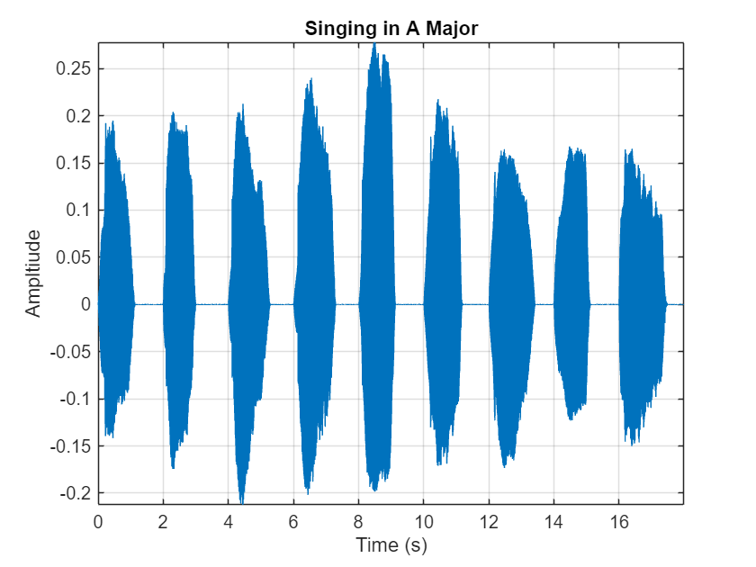
Read in an audio signal for pitch estimation. Visualize and listen to the audio. There are nine vocal utterances in the audio clip.
[audioIn,fs] = audioread('SingingAMajor-16-mono-18secs.ogg'); soundsc(audioIn,fs) T = 1/fs; t = 0:T:(length(audioIn)*T) - T; plot(t,audioIn); grid on axis tight xlabel('Time (s)') ylabel('Ampltiude') title('Singing in A Major')
Use crepePreprocess
to partition the audio into frames of 1024 samples with an 85% overlap between consecutive mel spectrograms. Place the frames along the fourth dimension.
[frames,loc] = crepePreprocess(audioIn,fs);
Create a CREPE network with ModelCapacity
set to tiny
. If you call crepe
before downloading the model, an error is printed to the Command Window with a download link.
netTiny = crepe('ModelCapacity','tiny');
Predict the network activations.
activationsTiny = predict(netTiny,frames);
Use crepePostprocess
to produce the fundamental frequency pitch estimation in Hz. Disable confidence thresholding by setting ConfidenceThreshold
to 0
.
f0Tiny = crepePostprocess(activationsTiny,'ConfidenceThreshold',0);
Visualize the pitch estimation over time.
plot(loc,f0Tiny) grid on axis tight xlabel('Time (s)') ylabel('Pitch Estimation (Hz)') title('CREPE Network Frequency Estimate - Thresholding Disabled')
With confidence thresholding disabled, crepePostprocess
provides a pitch estimate for every frame. Increase the ConfidenceThreshold
to 0.8
.
f0Tiny = crepePostprocess(activationsTiny,'ConfidenceThreshold',0.8);
Visualize the pitch estimation over time.
plot(loc,f0Tiny,'LineWidth',3) grid on axis tight xlabel('Time (s)') ylabel('Pitch Estimation (Hz)') title('CREPE Network Frequency Estimate - Thresholding Enabled')
Create a new CREPE network with ModelCapacity
set to full
.
netFull = crepe('ModelCapacity','full');
Predict the network activations.
activationsFull = predict(netFull,frames);
f0Full = crepePostprocess(activationsFull,'ConfidenceThreshold',0.8);
Visualize the pitch estimation. There are nine primary pitch estimation groupings, each group corresponding with one of the nine vocal utterances.
plot(loc,f0Full,'LineWidth',3) grid on xlabel('Time (s)') ylabel('Pitch Estimation (Hz)') title('CREPE Network Frequency Estimate - Full')
Find the time elements corresponding to the last vocal utterance.
roundedLocVec = round(loc,2); lastUtteranceBegin = find(roundedLocVec == 16); lastUtteranceEnd = find(roundedLocVec == 18);
For simplicity, take the most frequently occurring pitch estimate within the utterance group as the fundamental frequency estimate for that timespan. Generate a pure tone with a frequency matching the pitch estimate for the last vocal utterance.
lastUtteranceEstimation = mode(f0Full(lastUtteranceBegin:lastUtteranceEnd))
lastUtteranceEstimation = single
217.2709
The value for lastUtteranceEstimate
of 217.3
Hz. corresponds to the note A3. Overlay the synthesized tone on the last vocal utterance to audibly compare the two.
lastVocalUtterance = audioIn(fs*16:fs*18); newTime = 0:T:2; compareTone = cos(2*pi*lastUtteranceEstimation*newTime).'; soundsc(lastVocalUtterance + compareTone,fs);
Call spectrogram
to more closely inspect the frequency content of the singing. Use a frame size of 250
samples and an overlap of 225
samples or 90%. Use 4096
DFT points for the transform. The spectrogram
reveals that the vocal recording is actually a set of complex harmonic tones composed of multiple frequencies.
spectrogram(audioIn,250,225,4096,fs,'yaxis')
Input Arguments
audioIn
— Input signal
column vector | matrix
Input signal, specified as a column vector or matrix. If you specify a matrix,
crepePreprocess
treats the columns of the matrix as individual
audio channels.
Data Types: single
| double
fs
— Sample rate (Hz)
positive scalar
Sample rate of the input signal in Hz, specified as a positive scalar.
Data Types: single
| double
OP
— Overlap percentage between consecutive audio frames
85
(default) | nonnegative scalar in the range [0,100)
Percentage overlap between consecutive audio frames, specified as the
comma-separated pair consisting of 'OverlapPercentage'
and a scalar
in the range [0,100).
Data Types: single
| double
Output Arguments
frames
— Audio frames that can be fed to CREPE pretrained network
1024
-by-1
-by-1
-by-N
array
Processed audio frames, returned as a
1024
-by-1
-by-1
-by-N
array, where N is the number of generated frames.
Note
For multichannel inputs, generated frames
are stacked along
the 4th dimension according to channel. For example, if audioIn
is a stereo signal, the number of generated frames
for each
channel is actually N/2
. The first
N/2
frames
correspond to channel 1 and the subsequent
N/2
frames
correspond to channel 2.
Data Types: single
| double
loc
— Time values
1
-by-N vector
Time values associated with each frame, returned as a
1
-by-N vector, where N is the
number of generated frames. The time values correspond to the most recent samples used
to compute the frames.
Data Types: single
| double
References
[1] Kim, Jong Wook, Justin Salamon, Peter Li, and Juan Pablo Bello. “Crepe: A Convolutional Representation for Pitch Estimation.” In 2018 IEEE International Conference on Acoustics, Speech and Signal Processing (ICASSP), 161–65. Calgary, AB: IEEE, 2018. https://doi.org/10.1109/ICASSP.2018.8461329.
Extended Capabilities
C/C++ Code Generation
Generate C and C++ code using MATLAB® Coder™.
GPU Arrays
Accelerate code by running on a graphics processing unit (GPU) using Parallel Computing Toolbox™.
This function fully supports GPU arrays. For more information, see Run MATLAB Functions on a GPU (Parallel Computing Toolbox).
Version History
Introduced in R2021a
See Also
MATLAB 命令
您点击的链接对应于以下 MATLAB 命令:
请在 MATLAB 命令行窗口中直接输入以执行命令。Web 浏览器不支持 MATLAB 命令。
Select a Web Site
Choose a web site to get translated content where available and see local events and offers. Based on your location, we recommend that you select: .
You can also select a web site from the following list:
How to Get Best Site Performance
Select the China site (in Chinese or English) for best site performance. Other MathWorks country sites are not optimized for visits from your location.
Americas
- América Latina (Español)
- Canada (English)
- United States (English)
Europe
- Belgium (English)
- Denmark (English)
- Deutschland (Deutsch)
- España (Español)
- Finland (English)
- France (Français)
- Ireland (English)
- Italia (Italiano)
- Luxembourg (English)
- Netherlands (English)
- Norway (English)
- Österreich (Deutsch)
- Portugal (English)
- Sweden (English)
- Switzerland
- United Kingdom (English)