predictRT60

R2026b

Predict reverberation decay time of room

Since R2026b

collapse all in page

Syntax

t60 = predictRT60(room)

t60 = predictRT60(___,Name=Value)

predictRT60(___)

Description

Add-On Required: This feature requires the Room Acoustics Simulation add-on.

t60 = predictRT60(room) returns the predicted frequency-dependent reverberation decay time for the given room specification.

example

t60 = predictRT60(___,Name=Value) specifies options using one or more name-value arguments.

example

predictRT60(___) without any output arguments plots the predicted frequency-dependent decay time.

Examples

collapse all

Predict the RT-60 of a Shoebox Room

This example uses:

Open Live Script

Specify the dimensions in meters of a simple shoebox room. The first dimension is the length along the x-axis, the second dimension is the width along the y-axis, and the third dimension is the height along the z-axis.

roomDimensions = [5,4,6];

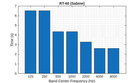
Plot the predicted decay time of the room using the Sabine formula.

predictRT60(roomDimensions)

Figure contains an axes object. The axes object with title RT-60 (Sabine), xlabel Band Center Frequency (Hz), ylabel Time (s) contains an object of type bar.

Predict RT-60 from a `triangulation` Object

This example uses:

Open Live Script

Predict the decay time of a room defined using a triangulation object where the surfaces are defined using materials from the acousticMaterialCatalog function.

Create a triangulation object representing a room.

roomDimensions = [5.5 4.5 4.2];
X = roomDimensions(1);
Y = roomDimensions(2);
Z = roomDimensions(3);
pts = [0 0 0;
    0 Y 0;
    X 0 0;
    X Y 0;
    0 0 Z;
    0 Y Z;
    X 0 Z;
    X Y Z];
dt = delaunayTriangulation(pts(:,1), pts(:,2), pts(:,3));
[conn,verts] = freeBoundary(dt);
scene = triangulation(conn, verts);

Specify the surface material as smooth, unpainted concrete and get RT-60 values using the Eyring formula.

t60 = predictRT60(scene,Method="eyring",MaterialAbsorption="SmoothUnpaintedConcrete")

t60 = 1×7 table
     125       250       500       1000      2000      4000      8000 
    ______    ______    ______    ______    ______    ______    ______

    12.482    12.482    6.2096    6.2096    6.2096    2.4458    1.5045

Compare RT-60 Formulas

This example uses:

Open Live Script

Predict the RT-60 of a given room using the Sabine, Eyring, Eyring-Kuttruff, and Modified Fitzroy formulas.

Specify the dimensions of a simple shoebox room.

room = [8, 10, 3.7];

Predict RT-60 for band center frequencies at 125 Hz, 250 Hz, 500 Hz, 1000 Hz, 2000 Hz, and 4000 Hz using each formula. Specify the room materials as a cork tile floor, painted plaster walls, and a drop ceiling.

bands = [125,250,500,1000,2000,4000];
floorMaterial = "CorkTileFloor";
wallMaterial = "PaintedPlaster";
ceilingMaterial = "OwensCorningDropCeiling";
materials = [floorMaterial,wallMaterial, ...
    wallMaterial,wallMaterial, ...
    wallMaterial,ceilingMaterial];
rt60_sabine = predictRT60(room, ...
    BandCenterFrequencies=bands, ...
    MaterialAbsorption=materials);
rt60_eyring = predictRT60(room, ...
    Method="eyring", ...
    BandCenterFrequencies=bands, ...
    MaterialAbsorption=materials);
rt60_eyringkuttruff = predictRT60(room, ...
    Method="eyring-kuttruff", ...
    BandCenterFrequencies=bands, ...
    MaterialAbsorption=materials);
rt60_fitzroy = predictRT60(room, ...
    Method="modified fitzroy", ...
    BandCenterFrequencies=bands, ...
    MaterialAbsorption=materials);

Plot the RT-60 values to compare the predictions.

xall = [rt60_sabine{:,:};rt60_eyring{:,:};rt60_eyringkuttruff{:,:};rt60_fitzroy{:,:}];  
bar(["125","250","500","1000","2000","4000"],xall)  
grid on  
ylabel("RT-60 (s)")  
xlabel("Octave Band Center Frequency (Hz)")  
legend("Sabine","Eyring","Eyring-Kuttruff","Modified-Fitzroy")  
title("Comparison of Predicted RT-60 Values")  
ylim([min(xall,[],"all")-0.1,max(xall,[],"all")+0.1])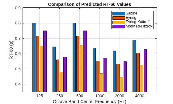

Figure contains an axes object. The axes object with title Comparison of Predicted RT-60 Values, xlabel Octave Band Center Frequency (Hz), ylabel RT-60 (s) contains 4 objects of type bar. These objects represent Sabine, Eyring, Eyring-Kuttruff, Modified-Fitzroy.

Analytical and Physical Modeling of RT-60

This example uses:

Open Live Script

In this example, you calculate reverberation time (RT-60) of a room using both the Sabine equation and a more physically accurate room modeling approach. In the first section, you use the Sabine equation to estimate RT-60 from room dimensions and absorption coefficients. Then you simulate the room impulse response (RIR) using physical modeling to obtain a more realistic RT-60. In the second section, you invert the Sabine equation to find absorption coefficients required to achieve a desired RT-60 in each frequency band. Finally, you compare the Sabine-predicted RT-60 values to physical modeling.

Sabine Equation

The Sabine equation is a classic analytical formula to estimate the reverberation time of an enclosed space based on its geometry and average surface absorption. The Sabine equation was published by Wallace Clement Sabine in 1900 after extensive experiments in the Fogg Lecture Hall at Harvard University. Sabine discovered that the reverberation time is proportional to the room's volume and inversely proportional to the total effective absorption:

${R T}_{60} = \frac{(55.25 / c) V}{A}$

where:

${R T}_{60}$ is the reverberation time in seconds.
$c$ is the speed of sound in meters per second.
$V$ is the room volume in cubic meters.
$A$ is the total absorption of room in metric sabins.

The Sabine equation is still in use today and is a valuable tool for its simplicity. However, it has several limitations, such as:

Assumes the sound field is perfectly diffuse--meaning a uniform distribution of sound energy throughout the room
Assumes absorption is evenly distributed on all surfaces
Is less accurate in small and irregular rooms
Does not account for air absorption, scattering, or diffraction effects
Can be inaccurate when the mean absorption coefficients are greater than 0.25

For the purposes of this example, the physical room and simulation are contrived to simulate many of the suppositions of the Sabine equation.

Room Modeling for RT-60 Estimation

Define room dimensions in meters. Choose dimensions that are not integer multiples of each other to avoid modal degeneracies in the physical simulation.

roomdims = [9.5,7.1,3.1]; % length, width, height

Specify absorption coefficients for six frequency bands: 125, 250, 500, 1000, 2000, and 4000 Hz. Use the same absorption coefficients on each surface of the room to follow Sabine's assumption of a diffuse acoustic field. The values are moderate and representative of mostly absorptive surfaces that one could find in a theater.

alpha = [0.2045,0.2100,0.1900,0.2097,0.2495,0.2835];

Use the Sabine equation to estimate the RT-60 for each frequency band.

t60_sabine = predictRT60(roomdims, ...
BandCenterFrequencies=[125,250,500,1000,2000,4000], ...
MaterialAbsorption=alpha)

t60_sabine = 1×6 table
      125        250        500       1000       2000       4000  
    _______    _______    _______    _______    _______    _______

    0.69268    0.67454    0.74555    0.67551    0.56775    0.49966

Isolate the RT-60 values for later comparison.

t60_sabine = table2array(t60_sabine);

Next, use a physical modeling approach to simulate the room's impulse response and estimate the RT-60 from the simulated data.

Define a sampling frequency for the simulation.

fs = 24e3;

Define source and receiver positions for the simulation. The height, 1.55 m, is roughly ear level and a common choice. To reduce the dominance of early reflections and to avoid strong room modes, the positions are away from the walls and corners.

sourceloc = [2.1,2.3,1.55];
receiverloc = [7.0,4.9,1.55];

Use high scattering coefficients to simulate a diffuse acoustic field. Use the same six frequency-dependent scattering coefficients for all surfaces.

scatteringCoeffs = [0.8,0.5,0.5,0.5,0.5,0.5];

To simulate the impulse response using a hybrid image-source and ray-tracing algorithm, use acousticRoomResponse. Use the default parameters of the stochastic ray tracing algorithm (MaxNumRayReflections=10 and NumStochasticRays=1280) to model the reverberant tail. Increase the image-source order for a more accurate model of the sound reflections.

ir = acousticRoomResponse(roomdims,sourceloc,receiverloc, ...
    BandCenterFrequencies=[125,250,500,1000,2000,4000], ...
    AirAbsorption=0, ...
    MaterialAbsorption=alpha, ...
    MaterialScattering=scatteringCoeffs, ...
    Algorithm="hybrid", ...
    MaxNumRayReflections=10, ...
    NumStochasticRays=1280, ...
    ImageSourceOrder=45);

To simulate a realistic measurement, add a noise floor to the impulse response. The supporting function iAddNoiseFloor does this.

noiseFloor = -80; % dB
rir = iAddNoiseFloor(ir,fs,noiseFloor);

Estimate the RT-60 from the simulated room impulse response using T30. RT-60 is the time it takes to the energy of an impulse response to decrease 60 dB from its peak. However, actually achieving a 60 dB dynamic range in a measurement is unlikely due to noise floors in most real measurements. Generally, a 20 dB range or 30 dB range (T20 and T30, respectively) is measured and the slope is extrapolated to 60 dB.

t60 = rt60(rir,fs,FilterOrder=64);
t60_physicalmodel = t60.T30'

t60_physicalmodel = 1×6

    0.7005    0.6877    0.7331    0.6720    0.5700    0.5028

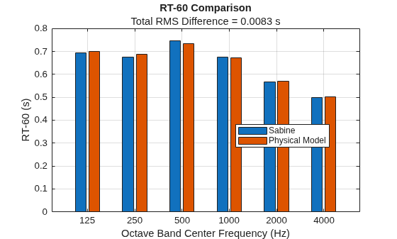
Compare the analytical (Sabine) and simulated (physical model) RT-60s by calculating their root mean square (RMS) difference. Display the RT-60 values and RMS difference.

rms_error = rms(t60_physicalmodel - t60_sabine);

figure
bar(["125","250","500","1000","2000","4000"],[t60_sabine(:),t60_physicalmodel(:)],"grouped");
xlabel("Octave Band Center Frequency (Hz)");
ylabel("RT-60 (s)");
legend("Sabine","Physical Model",Location="best");
title("RT-60 Comparison","Total RMS Difference = " + round(rms_error,4) + " s");
grid on

Figure contains an axes object. The axes object with title RT-60 Comparison, xlabel Octave Band Center Frequency (Hz), ylabel RT-60 (s) contains 2 objects of type bar. These objects represent Sabine, Physical Model.

Invert the Sabine Equation: Find Absorption Coefficients from Target RT-60

Assume you want to design the room to achieve specific target RT-60 values in each frequency band.

t60_target = [1,0.8,0.85,0.8,0.7,0.7];

Invert the Sabine equation to solve for the average absorption coefficient needed for each band. The supporting function iInverseRT60model does this.

alpha_target = iInverseRT60model(roomdims,t60_target)

alpha_target = 1×6

    0.1416    0.1770    0.1666    0.1770    0.2023    0.2023

Verify the resulting RT-60 values match the target values using the Sabine equation with the newly computed absorption coefficients.

t60_target_sabine = iRT60model(roomdims,alpha_target)

t60_target_sabine = 1×6

    1.0000    0.8000    0.8500    0.8000    0.7000    0.7000

Simulate the room again with these new absorption coefficients. Again, add a noise floor to simulate a realistic measurement.

ir = acousticRoomResponse(roomdims,sourceloc,receiverloc, ...
    BandCenterFrequencies=[125,250,500,1000,2000,4000], ...
    AirAbsorption=0, ...
    MaterialAbsorption=alpha_target, ...
    MaterialScattering=[0.8,0.5,0.5,0.5,0.5,0.5], ...
    Algorithm="hybrid", ...
    MaxNumRayReflections=10, ...
    NumStochasticRays=100, ...
    ImageSourceOrder=45);

noiseFloor = -80;
rir = iAddNoiseFloor(ir,fs,noiseFloor);

Estimate RT-60 from the simulated response.

t60 = rt60(rir,fs,FilterOrder=64);
t60_target_physicalmodel = t60.T30'

t60_target_physicalmodel = 1×6

    0.9325    0.9101    0.8583    0.7825    0.6921    0.6406

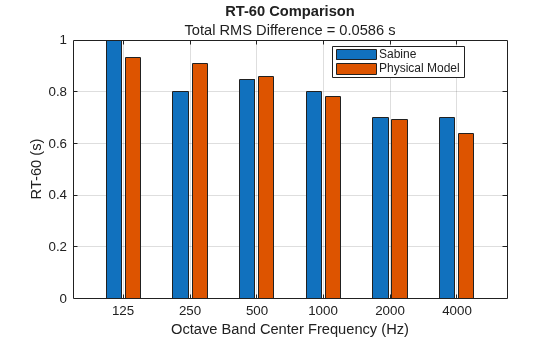
Compute the RMS error between the Sabine-predicted and simulated RT-60s and display the results.

rms_error = rms(t60_target_physicalmodel - t60_target_sabine);

figure
bar(["125","250","500","1000","2000","4000"],[t60_target_sabine(:),t60_target_physicalmodel(:)],"grouped");
xlabel("Octave Band Center Frequency (Hz)");
ylabel("RT-60 (s)");
legend("Sabine","Physical Model",Location="best");
title("RT-60 Comparison","Total RMS Difference = " + round(rms_error,4) + " s");
grid on

Supporting Functions

Add Noise Floor

function ir = iAddNoiseFloor(ir,fs,noiseFloor)
% Adds a pink noise floor to the impulse response to simulate measurement noise.

% Extend IR for ISO 3382 compliance (minimum 1.6 s duration)
flength = ceil(2*fs);

% Zero-pad IR to minimum length
if numel(ir) < flength
    ir = resize(ir(:),flength);
else
    ir = ir(:);
end

% Generate pink noise and normalize rms.
rng default
noise = pinknoise(numel(ir),1);
noise = noise./rms(noise);

% Scale pink noise to desired rms.
noise_rms = max(abs(ir(:))) * 10^(noiseFloor/20);
noise = noise*noise_rms;

ir = ir + noise;
end

RT-60 Model (Sabine)

function t60 = iRT60model(roomdims,alpha,options)
% Calculates RT-60 using the Sabine equation for a shoe-box room.
arguments
    roomdims
    alpha
    options.SoundSpeed (1,1) = 343 % (m/s)
end

Lx = roomdims(1); % Length
Ly = roomdims(2); % Width
Lz = roomdims(3); % Height

% Surface areas
Sxy = Lx*Ly;
Syx = Sxy;
Sxz = Lx*Lz;
Szx = Sxz;
Syz = Ly*Lz;
Szy = Syz;

S = [Sxy;Syx;Sxz;Szx;Syz;Szy];

% Total Volume
V = prod(roomdims);

% Compute the frequency-dependent effective absorbing area of the room surfaces.
A = sum(S.*alpha,1);

% Apply Sabine formula
t60 = (55.25/options.SoundSpeed)*V./A;
end

Inverse RT-60 Model (Sabine)

function alpha = iInverseRT60model(roomdims,t60,options)
% Inverts the Sabine equation to estimate the average absorption coefficient
% required to achieve a target RT-60 in each frequency band.
arguments
    roomdims
    t60
    options.SoundSpeed (1,1) = 343 % (m/s)
end

Lx = roomdims(1); % Length
Ly = roomdims(2); % Width
Lz = roomdims(3); % Height

% Surface areas
Sxy = Lx*Ly;
Syx = Sxy;
Sxz = Lx*Lz;
Szx = Sxz;
Syz = Ly*Lz;
Szy = Syz;

S = [Sxy;Syx;Sxz;Szx;Syz;Szy];

% Total Volume
V = prod(roomdims);

% Total surface area
Stot = sum(S);

% Invert Sabine formula:
alpha = (55.25/options.SoundSpeed).*V./ (Stot.*t60);
end

Input Arguments

collapse all

`room` — Room
1-by-3 vector | `triangulation` object

Room representation used to predict the decay time, specified as a 1-by-3 vector or a triangulation object. For a shoebox room, specify a 1-by-3 vector with dimensions L, W, and H, in meters, along the x-, y-, and z-axis, respectively.

predictRT60 supports triangulation objects with triangular faces. Tetrahedron meshes are not supported. You can create a triangulation object to represent the room directly by using triangulation, the freeBoundary function of a delaunayTriangulation object, or by reading in an STL file by using stlread.

Name-Value Arguments

collapse all

Specify optional pairs of arguments as Name1=Value1,...,NameN=ValueN, where Name is the argument name and Value is the corresponding value. Name-value arguments must appear after other arguments, but the order of the pairs does not matter.

Example: predictRT60(room,Method="eyring")

`Method` — Analytic formula
`"sabine"` (default) | `"eyring"` | `"eyring-kuttruff"` | `"modified fitzroy"`

Analytic formula used to predict the RT-60 of the room, specified as one of "sabine", "eyring", "eyring-kuttruff", or "modified fitzroy". The Modified Fitzroy formula is valid only when room is specified as a 1-by-3 vector. For more information on the available formulas, see More About.

Data Types: char | string

`MaterialAbsorption` — Material absorption coefficients
`[0.02,0.02,0.03,0.03,0.04,0.05,0.05]` (default) | numeric vector | matrix | string scalar | character vector | vector of strings | cell array of character vectors

Material absorption coefficients for room surfaces. The absorption coefficient describes the proportion of energy lost during reflection. Specify this argument as one of these values:

`MaterialAbsorption` value	Behavior
1-by-N numeric vector	Absorption coefficients in the range 0 to 1. N is the number of frequency bands specified by `BandCenterFrequencies`. Absorption coefficients apply to every surface or triangle of `room`.
string or character vector	Name of surface material. The value must match an entry in `acousticMaterialCatalog`. Absorption coefficients apply to every surface or triangle of `room`.
M-by-1 numeric vector	Absorption coefficients in the range 0 to 1. M is the number of surfaces or triangles of `room`. Each surface or triangle receives a single absorption coefficient that applies to all bands.
M-element string vector or cell array of character vectors	Name of surface material for each surface or triangle in `room`. The values must match entries in `acousticMaterialCatalog`.
M-by-N numeric matrix	Absorption coefficients in the range 0 to 1. M is the number of surfaces or triangles of `room`, and N is the number of frequency bands specified by `BandCenterFrequencies`.

When the material absorption coefficients are specified as a column vector or matrix:

If room represents a shoebox room with dimensions L, W, and H, the rows of MaterialAbsorption correspond to the surfaces of the room in this order: floor (z = 0), front (y = 0), back (y = W), left (x = 0), right (x = L), and ceiling (z = H).
If room is a triangulation object, the order of rows in MaterialAbsorption corresponds to the order of triangles in the ConnectivityList property of the triangulation object.

Data Types: single | double | string | char

`BandCenterFrequencies` — Center frequencies of bandpass filters
`[125,250,500,1000,2000,4000,8000]` (default) | positive vector

Center frequencies of the bandpass filters in Hz, specified as a vector of strictly increasing positive values.

Data Types: single | double

`AirAbsorption` — Air absorption coefficient
`0` (default) | scalar in range [0, 1] | vector

Air absorption coefficient in nepers per meter, specified as a scalar in the range 0 to 1. You can also specify this argument as a vector to define the air absorption coefficients for each of the frequencies in BandCenterFrequencies.

Data Types: single | double

`SoundSpeed` — Speed of sound
`343` (default) | positive scalar

Speed of sound in meters per second, specified as a positive scalar.

Data Types: single | double

Output Arguments

collapse all

`t60` — RT-60 prediction
table

RT-60 prediction, returned as a table with variable names equal to the center frequencies specified by BandCenterFrequencies and values as the predicted RT-60 in seconds for each band.

More About

collapse all

Shared Quantities Between Formulas

The formulas available in the predictRT60 function are computed using these quantities related to room dimensions and acoustic absorption:

c is the speed of sound in m/s.
k = 24ln(10)/c is the Sabine constant.
V is the room volume in m³.
m is the air absorption coefficient. When AirAbsorption is specified as a vector, m can be different for each frequency band.
S_i is the surface area of the ith surface in m².
S = Σ S_i is the total surface area in m².
α_i is the per-band material absorption coefficients of the ith surface.
A = Σ S_iα_i is the total absorption in sabins per band.
α = A/S is the per-band average absorption.
ρ_i = 1–α_i is the per-band reflection coefficients of the ith surface.
ρ = 1–α is the per-band average reflection.

Sabine Formula

The Sabine formula [1] estimates the decay time as

$T_{60} = \frac{k V}{A + 4 m V} .$

Eyring Formula

The Eyring formula [1] (sometimes referred to as the Norris-Eyring or Eyring-Norris formula) estimates the decay time as

$T_{60} = \frac{k V}{- S \ln (ρ) + 4 m V} .$

Eyring-Kuttruff Formula

The Eyring-Kuttruff formula [2] adds the corrective term

$Δ = S \cdot (\frac{\sum_{i} ρ_{i} (ρ_{i} - ρ) \cdot S_{i}^{2}}{{(ρ S)}^{2} - \sum_{i} (ρ_{i}^{2} \cdot S_{i}^{2})})$

to the denominator of the Eyring formula, estimating decay time as

$T_{60} = \frac{k V}{- S \ln (ρ) + Δ + 4 m V} .$

Modified Fitzroy Formula

The Modified Fitzroy formula [2] is valid only for shoebox rooms defined by height H, length L, and width W. The formula calculates area weighted absorption coefficients α^*_WW and α^*_CF to calculate an effective absorption area as

$\begin{array}{l} d_{eff} = \frac{2 L H + 2 H W}{α_{WW}^{*}} + \frac{2 L W}{α_{CF}^{*}}, \\ A_{eff} = \frac{{(2 H (L + W) + 2 L W)}^{2}}{d_{eff}} . \end{array}$

The decay time is estimated as

$T_{60} = \frac{k V}{A_{eff} + 4 m V} .$

References

[1] Everest, Frederick A., and Ken C. Pohlmann. Master Handbook of Acoustics. 7. ed. McGraw-Hill, 2021.

[2] Neubauer, Reinhard O. “Estimation of Reverberation Time in Rectangular Rooms with Non-Uniformly Distributed Absorption Using a Modified Fitzroy Equation.” Building Acoustics 8, no. 2 (2001): 115–37. https://doi.org/10.1260/1351010011501786.

Extended Capabilities

expand all

C/C++ Code Generation
Generate C and C++ code using MATLAB® Coder™.

Usage notes and limitations:

Code generation is only supported for shoebox rooms. If MaterialAbsorption is specified as a cell array of character vectors, it must be constant at compile time.

Version History

Introduced in R2026b

predictRT60

Syntax

Description

Examples

Predict the RT-60 of a Shoebox Room

Predict RT-60 from a `triangulation` Object

Compare RT-60 Formulas

Analytical and Physical Modeling of RT-60

Input Arguments

`room` — Room
1-by-3 vector | `triangulation` object

Name-Value Arguments

`Method` — Analytic formula
`"sabine"` (default) | `"eyring"` | `"eyring-kuttruff"` | `"modified fitzroy"`

`MaterialAbsorption` — Material absorption coefficients
`[0.02,0.02,0.03,0.03,0.04,0.05,0.05]` (default) | numeric vector | matrix | string scalar | character vector | vector of strings | cell array of character vectors

`BandCenterFrequencies` — Center frequencies of bandpass filters
`[125,250,500,1000,2000,4000,8000]` (default) | positive vector

`AirAbsorption` — Air absorption coefficient
`0` (default) | scalar in range [0, 1] | vector

`SoundSpeed` — Speed of sound
`343` (default) | positive scalar

Output Arguments

`t60` — RT-60 prediction
table

More About

Shared Quantities Between Formulas

Sabine Formula

Eyring Formula

Eyring-Kuttruff Formula

Modified Fitzroy Formula

References

Extended Capabilities

C/C++ Code Generation
Generate C and C++ code using MATLAB® Coder™.

Version History

See Also

Topics

predictRT60

Syntax

Description

Examples

Predict the RT-60 of a Shoebox Room

Predict RT-60 from a triangulation Object

Compare RT-60 Formulas

Analytical and Physical Modeling of RT-60

Input Arguments

room — Room 1-by-3 vector | triangulation object

Name-Value Arguments

Method — Analytic formula "sabine" (default) | "eyring" | "eyring-kuttruff" | "modified fitzroy"

MaterialAbsorption — Material absorption coefficients [0.02,0.02,0.03,0.03,0.04,0.05,0.05] (default) | numeric vector | matrix | string scalar | character vector | vector of strings | cell array of character vectors

BandCenterFrequencies — Center frequencies of bandpass filters [125,250,500,1000,2000,4000,8000] (default) | positive vector

AirAbsorption — Air absorption coefficient 0 (default) | scalar in range [0, 1] | vector

SoundSpeed — Speed of sound 343 (default) | positive scalar

Output Arguments

t60 — RT-60 prediction table

More About

Shared Quantities Between Formulas

Sabine Formula

Eyring Formula

Eyring-Kuttruff Formula

Modified Fitzroy Formula

References

Extended Capabilities

C/C++ Code Generation Generate C and C++ code using MATLAB® Coder™.

Version History

See Also

Topics

Predict RT-60 from a `triangulation` Object

`room` — Room
1-by-3 vector | `triangulation` object

`Method` — Analytic formula
`"sabine"` (default) | `"eyring"` | `"eyring-kuttruff"` | `"modified fitzroy"`

`MaterialAbsorption` — Material absorption coefficients
`[0.02,0.02,0.03,0.03,0.04,0.05,0.05]` (default) | numeric vector | matrix | string scalar | character vector | vector of strings | cell array of character vectors

`BandCenterFrequencies` — Center frequencies of bandpass filters
`[125,250,500,1000,2000,4000,8000]` (default) | positive vector

`AirAbsorption` — Air absorption coefficient
`0` (default) | scalar in range [0, 1] | vector

`SoundSpeed` — Speed of sound
`343` (default) | positive scalar

`t60` — RT-60 prediction
table

C/C++ Code Generation
Generate C and C++ code using MATLAB® Coder™.