Acoustics-Based Machine Fault Recognition Code Generation on Raspberry Pi
This example demonstrates code generation for Acoustics-Based Machine Fault Recognition using a long short-term memory (LSTM) network and spectral descriptors. This example uses MATLAB® Coder™, MATLAB Coder Interface for Deep Learning, Raspberry Pi® Blockset to generate a standalone executable (.elf) file on a Raspberry Pi. The input data consists of acoustics time-series recordings from faulty or healthy air compressors and the output is the state of the mechanical machine predicted by the LSTM network. This standalone executable on Raspberry Pi runs the streaming classifier on the input data received from MATLAB and sends the computed scores for each label to MATLAB. Interaction between MATLAB script and the executable on your Raspberry Pi is handled using the user datagram protocol (UDP). For more details on audio preprocessing and network training, see Acoustics-Based Machine Fault Recognition.
Prepare Input Dataset
Specify a sample rate fs of 16 kHz and a windowLength of 512 samples, as defined in Acoustics-Based Machine Fault Recognition. Set numFrames to 100.
fs = 16000;
windowLength = 512;
numFrames = 100;
To run the example on a test signal, generate a pink noise signal. To test the performance of the system on a real dataset, download the air compressor dataset [1].
downloadDataset =true; if ~downloadDataset pinkNoiseSignal = pinknoise(windowLength*numFrames,1,"single"); else % Download AirCompressorDataset.zip component = 'audio'; filename = 'AirCompressorDataset/AirCompressorDataset.zip'; localfile = matlab.internal.examples.downloadSupportFile(component,filename); % Unzip the downloaded zip file to the downloadFolder downloadFolder = fileparts(localfile); if ~exist(fullfile(downloadFolder,'AirCompressorDataset'),'dir') unzip(localfile, downloadFolder) end % Create an audioDatastore object dataStore, to manage, the data. dataStore = audioDatastore(downloadFolder, ... IncludeSubfolders=true, ... LabelSource="foldernames", ... OutputDataType="single"); % Use countEachLabel to get the number of samples of each category in the dataset. countEachLabel(dataStore) end
ans=8×2 table
      Bearing    225
     Flywheel    225
      Healthy    225
          LIV    225
          LOV    225
          NRV    225
       Piston    225
    Riderbelt    225
Streaming Demonstration in MATLAB
To run the streaming classifier in MATLAB, load the system developed in Acoustics-Based Machine Fault Recognition.
load("AirCompressorFaultRecognitionModel.mat","airCompNet","labels");
Create a dsp.AsyncBuffer object to read audio in a streaming fashion and a dsp.AsyncBuffer object to accumulate scores.
audioSource = dsp.AsyncBuffer;
scoreBuffer = dsp.AsyncBuffer;
Initialize signalToBeTested to pinkNoiseSignal or select a signal from the drop-down list to test the file of your choice from the dataset.
if ~downloadDataset signalToBeTested = pinkNoiseSignal; else [allFiles,~] = splitEachLabel(dataStore,1); allData = readall(allFiles); signalToBeTested =allData(7); signalToBeTested = cell2mat(signalToBeTested); end
Stream one audio frame at a time to represent the system as it would be deployed in a real-time embedded system. Use recognizeAirCompressorFault developed in Acoustics-Based Machine Fault Recognition to compute audio features and perform deep learning classification.
reset(audioSource)
write(audioSource,signalToBeTested);
resetNetworkState = true;

while audioSource.NumUnreadSamples >= windowLength

    % Get a frame of audio data
    x = read(audioSource,windowLength);

    % Apply streaming classifier function
    score = recognizeAirCompressorFault(x,resetNetworkState);

    % Store score for analysis
    write(scoreBuffer,extractdata(score)');

    resetNetworkState = false;
end
Compute the recognized fault from scores and display it.
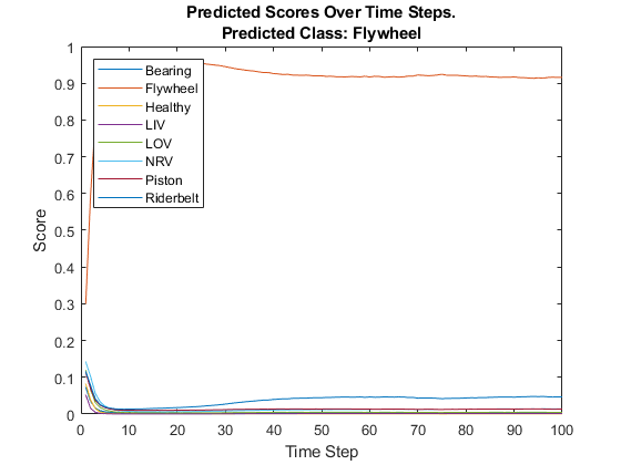
scores = read(scoreBuffer);
[~,labelIndex] = max(scores(end,:),[],2);
detectedFault = labels(labelIndex)
detectedFault = categorical
     Piston
Plot the scores of each label for each frame.
plot(scores)
legend(string(labels),Location="northwest")
xlabel("Time Step")
ylabel("Score")
str = sprintf("Predicted Scores Over Time Steps.\nPredicted Class: %s",detectedFault);
title(str)
Reset the asynchronous buffer audioSource.
reset(audioSource)
Prepare MATLAB Code For Deployment
Create a supporting function, recognizeAirCompressorFaultRaspi, that receives an audio frame using dsp.UDPReceiver and applies the streaming classifier and sends the predicted score vector to MATLAB using dsp.UDPSender.
type recognizeAirCompressorFaultRaspifunction recognizeAirCompressorFaultRaspi(hostIPAddress)
% This function receives acoustic input using dsp.UDPReceiver and runs a
% streaming classifier by calling recognizeAirCompressorFault, developed in
% the Acoustics-Based Machine Fault Recognition - MATLAB Example.
% Computed scores are sent to MATLAB using dsp.UDPSender.
%#codegen
% Copyright 2021-2025 The MathWorks, Inc.
frameLength = 512;
% Configure UDP Sender System Object
UDPSend = dsp.UDPSender( ...
RemoteIPPort=21000, ...
RemoteIPAddress=hostIPAddress);
% Configure UDP Receiver system object
sizeOfSingleInBytes = 4;
maxUDPMessageLength = floor(65507/sizeOfSingleInBytes);
numPackets = floor(maxUDPMessageLength/frameLength);
bufferSize = numPackets*frameLength*sizeOfSingleInBytes;
UDPReceiveRaspi = dsp.UDPReceiver( ...
LocalIPPort=25000, ...
MaximumMessageLength=frameLength, ...
ReceiveBufferSize=bufferSize, ...
MessageDataType='single');
% Reset network state for first call
resetNetworkState = true;
while true
% Receive audio frame of size frameLength x 1
x = UDPReceiveRaspi();
if(~isempty(x))
x = x(1:frameLength,1);
% Apply streaming classifier function
scores = recognizeAirCompressorFault(x,resetNetworkState);
% Send output to the host machine
UDPSend(single(scores));
resetNetworkState = false;
end
end
Generate Executable on Raspberry Pi
Replace the hostIPAddress with your machine's address. Your Raspberry Pi sends the predicted scores to the IP address you specify.
hostIPAddress = coder.Constant("********");Create a code generation configuration object to generate an executable program. Specify the target language as C.
cfg = coder.config("exe");
cfg.TargetLang = "C";
Use the Raspberry Pi® Blockset function, raspi, to create a connection to your Raspberry Pi. In the following code, replace:
targetIPAddresswith the IP address of your Raspberry Piusernamewith your user namepasswordwith your password
targetIPAddress = "********";
username = "********";
password = "********";
r = raspi(targetIPAddress,username,password);
Create a coder.hardware (MATLAB Coder) object for Raspberry Pi and attach it to the code generation configuration object.
hw = coder.hardware("Raspberry Pi");
hw.DeviceAddress = targetIPAddress;
hw.Username = username;
hw.Password = password;

cfg.Hardware = hw;
Specify the build folder on the Raspberry Pi.
buildDir = '~/remoteBuildDir';
cfg.Hardware.BuildDir = buildDir;

cfg.LargeConstantGeneration = "WriteOnlyDNNConstantsToDataFiles";
cfg.LargeConstantThreshold = 1024;
Use an auto generated C main file for the generation of a standalone executable.
cfg.GenerateExampleMain = "GenerateCodeAndCompile";Call the codegen (MATLAB Coder) function from to generate C code and the executable on your Raspberry Pi. By default, the Raspberry Pi application name is the same as the MATLAB function. You get a warning in the code generation logs that you can disregard because recognizeAirCompressorFaultRaspi has an infinite loop that looks for an audio frame from MATLAB.
codegen recognizeAirCompressorFaultRaspi -config cfg -args {hostIPAddress} -report
Set Up UDP Communication
Create a dsp.UDPSender System object™ to send audio captured in MATLAB to your Raspberry Pi. Raspberry Pi receives the captured audio from the same port using the dsp.UDPReceiver System object.
UDPSend = dsp.UDPSender( ...
    RemoteIPPort=25000, ...
    RemoteIPAddress=targetIPAddress);
Create a dsp.UDPReceiver system object to receive predicted scores from your Raspberry Pi. Each UDP packet received from the Raspberry Pi is a vector of scores and each vector element is a score for a state of the air compressor. The maximum message length for the dsp.UDPReceiver object is 65507 bytes. Calculate the buffer size to accommodate the maximum number of UDP packets.
sizeOfFloatInBytes = 4;
numScores = 8;
maxUDPMessageLength = floor(65507/sizeOfFloatInBytes);
numPackets = floor(maxUDPMessageLength/numScores);
bufferSize = numPackets*numScores*sizeOfFloatInBytes;

UDPReceive = dsp.UDPReceiver( ...
    LocalIPPort=21000, ...
    MessageDataType="single", ...
    MaximumMessageLength=numScores, ...
    ReceiveBufferSize=bufferSize);
Initialize Application on Raspberry Pi
Create a command to open the recognizeAirCompressorFaultRaspi application on a Raspberry Pi. Use system to send the command to your Raspberry Pi.
applicationName = 'recognizeAirCompressorFaultRaspi';

applicationDirPaths = raspi.utils.getRemoteBuildDirectory(applicationName=applicationName);
targetDirPath = applicationDirPaths{1}.directory;

exeName = strcat(applicationName,'.elf');
command = ['cd ',targetDirPath,'; ./',exeName,' &> 1 &'];

system(r,command);
Perform Machine Fault Recognition Using Deployed Code
Initialize signalToBeTested to pinkNoiseSignal or select a signal from the drop-down list to test the file of your choice from the dataset.
if ~downloadDataset signalToBeTested = pinkNoiseSignal; else [allFiles,~] = splitEachLabel(dataStore,1); allData = readall(allFiles); signalToBeTested =allData(3); signalToBeTested = cell2mat(signalToBeTested); end
Stream one audio frame at a time to represent a system as it would be deployed in a real-time embedded system. Use the generated file to compute audio features and perform deep learning classification.
write(audioSource,signalToBeTested);

while audioSource.NumUnreadSamples >= windowLength
    x = read(audioSource,windowLength);
    UDPSend(single(x));
    score = UDPReceive();
    if ~isempty(score)
        write(scoreBuffer,score');
    end
end
Compute the recognized fault from scores and display it.
scores = read(scoreBuffer);
[~,labelIndex] = max(scores(end,:),[],2);
detectedFault = labels(labelIndex)
detectedFault = categorical
     Healthy
Plot the scores of each label for each frame.
plot(scores)
legend(string(labels),Location="northwest")
xlabel("Time Step")
ylabel("Score")
str = sprintf("Predicted Scores Over Time Steps.\nPredicted Class: %s",detectedFault);
title(str)

Terminate the standalone executable running on Raspberry Pi.
stopExecutable(codertarget.raspi.raspberrypi,exeName)
Profile Using PIL Workflow
To evaluate execution time taken by standalone executable on Raspberry Pi, use a PIL (processor-in-loop) workflow. To perform PIL profiling, generate a PIL function for the supporting function recognizeAirCompressorFault.
Create a code generation configuration object to generate the PIL function.
cfg = coder.config("lib",ecoder=true);
cfg.VerificationMode = "PIL";

cfg.Hardware = hw;
cfg.Hardware.BuildDir = buildDir;
cfg.TargetLang = "C";

cfg.LargeConstantGeneration = "WriteOnlyDNNConstantsToDataFiles";
cfg.LargeConstantThreshold = 1024;
Enable profiling and generate the PIL code. A MEX file named recognizeAirCompressorFault_pil is generated in your current folder.
cfg.CodeExecutionProfiling = true;
audioFrame = ones(windowLength,1,"single");
resetNetworkStateFlag = true;
codegen -config cfg recognizeAirCompressorFault -args {audioFrame,resetNetworkStateFlag} -report -v
Call the generated PIL function 50 times to get the average execution time.
totalCalls = 50;
x = pinknoise(windowLength,1,"single");

for k = 1:totalCalls
    score = recognizeAirCompressorFault_pil(x,resetNetworkStateFlag);
    resetNetworkStateFlag = false;
end
Terminate the PIL execution.
clear recognizeAirCompressorFault_pilGenerate an execution profile report to evaluate execution time.
executionProfile = getCoderExecutionProfile("recognizeAirCompressorFault");
report(executionProfile, ...
       Units="Seconds", ...
       ScaleFactor="1e-03", ...
       NumericFormat="%0.4f");


The average execution time of recognizeAirCompressorFault_pil function is 0.423 ms, which is well below the 32 ms budget for real-time performance. The first call of recognizeAirCompressorFault_pil consumes around 12 times of the average execution time as it includes loading of network and resetting of the states. However, in a real, deployed system, that initialization time is incurred only once. This example ends here. For deploying machine fault recognition on desktops, see Acoustics-Based Machine Fault Recognition Code Generation.
References
[1] Verma, Nishchal K., et al. "Intelligent Condition Based Monitoring Using Acoustic Signals for Air Compressors." IEEE Transactions on Reliability, vol. 65, no. 1, Mar. 2016, pp. 291–309. DOI.org (Crossref), doi:10.1109/TR.2015.2459684.