Evaluate Electric Vehicle Thermal Controller Performance

Configure Simscape Test Harness

Create and open a working copy of the electric vehicle thermal management system harness. This model uses constant heat-flow rates for the battery, motor, and DC-DC converter, which is useful for evaluating the controller and plant models under steady-state, controlled conditions. For more information on the thermal plant model, see Electric Vehicle Thermal Management with Heat Pump (Simscape Fluids).

currDir = pwd;
addpath(currDir);

autoblkThermalStart('constant');

Configure Model and Environment

Define the model, environment block, and controller block paths.

mdl = 'ThermalHarnessExample';
envBlk = [mdl '/Environment'];
ctrlBlk = 'ThermalControl/Controller';

Configure the model to use a stiff variable-step solver with tight tolerances and a reduced step size to prevent step-size warnings.

set_param(mdl, ...
    'Solver',      'daessc', ...
    'RelTol',      '1e-4',   ...
    'AbsTol',      '1e-6',   ...
    'StopTime',    '1500');

load_system(mdl);
load_system('ThermalControl');
load_system(ctrlBlk);

Define three ambient temperature scenarios that reflect the real-world operating envelope.

ambientTemps_C = [0 20 35];
numTemps = numel(ambientTemps_C);

Create a Simulink.SimulationInput array with one entry for each ambient condition. Each entry updates the Temperature parameter in the Environment block mask before each simulation. The Environment block also sets the atmospheric pressure, relative humidity, and CO2 fraction, which remain constant across all scenarios.

Enable Simscape logging on each run so that heat flow and power signals are available for COP analysis.

simIn(1:numTemps) = Simulink.SimulationInput(mdl);
for idx = 1:numTemps
    simIn(idx) = simIn(idx).setBlockParameter(envBlk, 'Temp', num2str(ambientTemps_C(idx),'%.15g'));
    simIn(idx) = simIn(idx).setModelParameter('SimscapeLogType', 'all');
end

Save any unsaved data dictionary and model changes so they are available on parallel workers.

dicts = Simulink.data.dictionary.getOpenDictionaryPaths;
for iDict = 1:numel(dicts)
    dd = Simulink.data.dictionary.open(dicts{iDict});
    if dd.HasUnsavedChanges
        dd.saveChanges;
    end
end
save_system('ThermalHarnessExample');

Run Simulations in Parallel

Use the parsim function to run all ambient scenarios in parallel. The parsim function requires Parallel Computing Toolbox™ for parallel execution but falls back to serial execution if the toolbox is not available.

simOut = parsim(simIn, 'ShowProgress', 'on');

Extract Simulation Results

Each Simulink.SimulationOutput object contains a simout structure with the logged signals. Extract these structures for plotting and analysis.

S = cell(1, numTemps);
for idx = 1:numTemps
    S{idx} = simOut(idx).simout;
end

Programmatically get the cabin, battery, and motor target temperatures from the controller block using slResolve and get_param. The controller stores targets in Kelvin. Convert to Celsius to match the logged measurement signals.

CabTrgT_C     = slResolve(get_param(ctrlBlk,'CabTrgT'),     ctrlBlk) - 273.15;
BattTrgTemp_C = slResolve(get_param(ctrlBlk,'BattTrgTemp'), ctrlBlk) - 273.15;
EMTrgTemp_C   = slResolve(get_param(ctrlBlk,'EMTrgTemp'),   ctrlBlk) - 273.15;

Compare Component Temperatures Against Targets

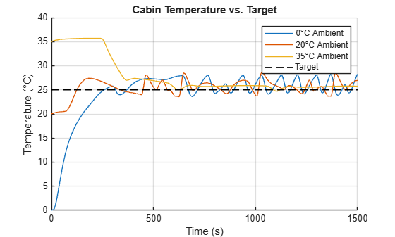
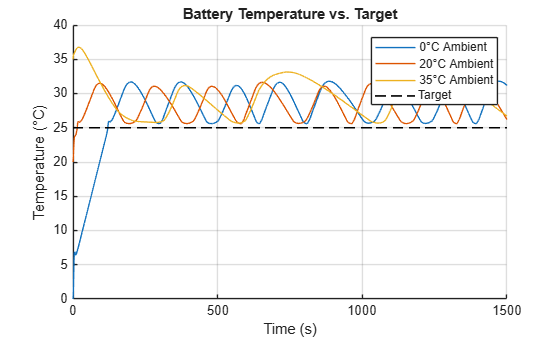
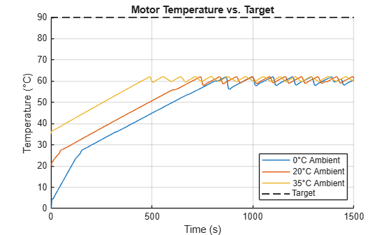
Before extracting efficiency numbers, verify the controller successfully regulates all components to their setpoints. If temperatures diverge from targets, the COP calculation reflects a fault condition, not a design characteristic. The plots in this section confirm the controller reaches steady-state regulation at all three ambient conditions.

labels = arrayfun(@(t) sprintf('%g\\circC Ambient', t), ambientTemps_C, 'UniformOutput', false);

Cabin Temperature

The cabin temperature is the most visible indicator of occupant comfort. The controller modulates the heating, ventilation, and air conditioning (HVAC) system to drive cabin temperature toward the target.

figure('Name','Cabin Temperature vs. Target');
plotCompare(S, 'CabinTemperature_C', CabTrgT_C, labels);
ylabel('Temperature (\circC)');
xlabel('Time (s)');
title('Cabin Temperature vs. Target');

Battery Temperature

Battery temperature directly affects cell longevity and charge acceptance. The controller uses the chiller loop and battery heater to maintain the battery within its optimal thermal window.

figure('Name','Battery Temperature vs. Target');
plotCompare(S, 'BattTemperature_C', BattTrgTemp_C, labels);
ylabel('Temperature (\circC)');
xlabel('Time (s)');
title('Battery Temperature vs. Target');

Motor Temperature

The electric motor generates waste heat proportional to its power output. The controller uses the radiator and coolant pumps to keep motor temperature below its derating threshold.

figure('Name','Motor Temperature vs. Target');
plotCompare(S, 'MotorTemperature_C', EMTrgTemp_C, labels);
ylabel('Temperature (\circC)');
xlabel('Time (s)');
title('Motor Temperature vs. Target');

Compare Controller Commands

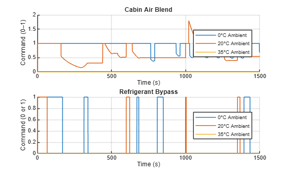
The controller commands show which actuators dominate the electrical budget at each condition. At 0 deg C, the PTC heater runs continuously. At 35 deg C, the compressor and fan work at capacity. The cabin air blend shows proportional actuation effort, while the refrigerant bypass reveals mode switching between heating and cooling.

figure('Name','Controller Commands');
subplot(2,1,1)
plotSignalCompare(S, 'BlndAirCmd', labels);
ylabel('Command (0–1)');
xlabel('Time (s)');
title('Cabin Air Blend');
subplot(2,1,2)
plotSignalCompare(S, 'RfrgByPCmd', labels);
ylabel('Command (0 or 1)');
xlabel('Time (s)');
title('Refrigerant Bypass');

Compute and Visualize System-Level COP

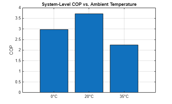
System-level COP accounts for all thermal actuators operating together under controller direction. Unlike a component-level COP from a datasheet, you can measure system-level COP only from the complete system, not derived from individual component specifications.

COP is defined as the ratio of total managed thermal load to total electrical work consumed by all thermal actuators. The numerator includes both cooling (heat removed from components) and heating (heat delivered to components). Some component heat flows are negative depending on operating mode. For example, the inner condenser Q is negative because it rejects refrigerant heat into the cabin, while the evaporator Q is positive because it absorbs cabin heat into the refrigerant. The extractCOP helper function uses absolute values so that both directions contribute positively to the total managed load.

Use the extractCOP helper function to navigate the Simscape logging hierarchy and compute time-averaged heat loads, electrical work, and COP for each simulation run.

cop = extractCOP(simOut, mdl);
Q_managed = cop.Q_managed;
W_total = cop.W_total;
COP_all = cop.COP;

Display the computed COP values alongside the heat loads and work inputs.

resultsTable = table(ambientTemps_C(:), COP_all(:), ...
    Q_managed(:), W_total(:), ...
    VariableNames=["AmbientTemp_C", "COP", "Q_Managed_W", "W_Total_W"])

resultsTable = 3×4 table
     0    2.9767    7.6801e+03    2.5800e+03
    20    3.7210    6.0710e+03    1.6315e+03
    35    2.2413    6.5655e+03    2.9293e+03

Visualize the measured COP at each ambient temperature.

figure('Name','System-Level COP vs. Ambient Temperature')
bar(categorical(string(ambientTemps_C) + "\circC"), COP_all(:))
ylabel('COP')
title('System-Level COP vs. Ambient Temperature')
grid on

Build COP Lookup Table

Package the COP values as a lookup table for vehicle-level range analysis. Each entry pairs an ambient temperature with the system efficiency measured at that condition.

copLookupTable.ambientTemp_degC = ambientTemps_C;
copLookupTable.COP = COP_all;
copLookupTable.Q_managed_W = Q_managed;
copLookupTable.W_total_W = W_total;
copLookupTable.metadata.source = 'ThermalHarnessExample (Simscape)';
copLookupTable.metadata.date = char(datetime('today'));
copLookupTable.metadata.description = 'Measured COP from Simscape thermal model at steady-state';
save('cop_lookup_table.mat', 'copLookupTable');
fprintf('Saved cop_lookup_table.mat with COP values for %d ambient temperatures.\n', numTemps);

Saved cop_lookup_table.mat with COP values for 3 ambient temperatures.

Next Steps

The cop_lookup_table.mat file contains the system-level COP at each ambient temperature. You can use this file as an input to vehicle-level simulations or as a baseline for further controller development.