Bluetooth LE Positioning with Deep Learning

Since R2024b

This example uses:

This example shows how to calculate the 3-D positioning of a Bluetooth® low energy (LE) node by using received signal strength indicator (RSSI) fingerprinting and a convolutional neural network (CNN). Using this example, you can:

Generate Bluetooth LE locator and node positions in an indoor environment.
Compute propagation paths between the nodes and locators in the indoor environment by using the ray tracing propagation model.
Create an RSSI fingerprint base for every node-locator pair.
Train the CNN model using the RSSI data set.
Evaluate and visualize the performance of the network by comparing the node positions predicted by the CNN with the actual positions.

You can further explore this example to see how you can improve the accuracy of the node positioning estimate by increasing the number of Bluetooth LE nodes for training. For more information, see Further Exploration.

Fingerprinting and Deep Learning in Bluetooth-Location Based Services

Bluetooth technology provides various types of location-based services [1], which fall into these two categories:

Proximity Solutions: Bluetooth proximity solutions estimate the distance between two devices by using received signal strength indication (RSSI) measurements.
Positioning Systems: Bluetooth positioning systems employ trilateration, using multiple RSSI measurements to pinpoint a device's location.

The introduction of new direction-finding features in the Bluetooth Core Specification 5.3 [2] enables you to estimate the location of a device with centimeter-level accuracy.

Bluetooth LE positioning systems can use fingerprinting and deep learning techniques to achieve sub-meter level accuracies, even in non-line-of-sight (NLOS) multipath environments [3]. A fingerprint typically includes information like the RSSI from a signal measured at a specific location within an environment.

The example performs these steps to estimate the 3-D position of a Bluetooth LE node by using RSSI and CNN.

Initiate the network's training phase by computing RSSI fingerprints at various known positions within an indoor environment.
Create a data set by collecting RSSI fingerprints from the received LE signals in an indoor environment, and label each fingerprint with its specific location information. Each fingerprint includes RSSI values derived from several LE packets from each transmitter locator.
Train a CNN to predict node locations using a subset of these fingerprints.
Assess the performance of the trained model by using the remainder of the data set to generate predictions of node locations based on their RSSI fingerprints.

Generate Training Data for Indoor Environment

Generate training data for an indoor office environment, specified by the conferenceroom.stl file.

mapFileName = "conferenceroom.stl";
viewer = siteviewer(SceneModel=mapFileName,Transparency=0.25);

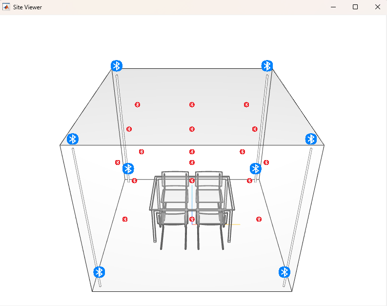
The example places $N_{locator}$ LE transmitters at corners of the room, and a number of receiving nodes that you specify in the environment. The example generates LE signals with 5 dBm output power, and computes the fingerprints based on the propagation channel that the environment defines.

This section shows how you can synthesize the training data set for the CNN.

Generate LE Locators and Node Positions in Indoor Environment

Generate the LE locators and node objects, and visualize them in the indoor scenario. If you use a file other than conferenceroom.stl to create the environment, you must adjust the locator and node positions in the createScenario function to accommodate the new environment. The example calculates the number of nodes by using the nodeSeparation value, which specifies the distance in meters between the nodes across all dimensions.

nodeSeparation = 1;                                              
[locators,nodes,posnodes] = createScenario(nodeSeparation);

show(locators,Icon="bleTxIcon.png")
show(nodes,Icon="bleRxIcon.png",ShowAntennaHeight=false,IconSize=[16 16])
disp("Simulating a scenario with " + num2str(width(locators)) + " locators and " + num2str(width(nodes)) + " nodes")

Simulating a scenario with 8 locators and 18 nodes

Generate Channel Characteristics by Using Ray Tracing Techniques

Set the parameters for the ray propagation model. This example considers only LOS and second-order reflections by specifying the MaxNumReflections input as 2. Increasing the MaxNumReflections value extends the simulation time.

pm = propagationModel("raytracing", ...
    CoordinateSystem="cartesian", ...
    SurfaceMaterial="wood", ...
    MaxNumReflections=2);

Perform ray tracing analysis for all the locator-node pairs. The raytrace function returns the generated rays in a cell array of size $N_{beacon}$ -by- $N_{node}$ , where $N_{beacon}$ is the number of locators and $N_{node}$ is the number of nodes.

rays = raytrace(locators,nodes,pm,"Map",mapFileName);

Visualize the propagation paths between all locators and a single node. A distinct color specifies the path loss in dB associated with each reflected path.

hide(nodes);
show(nodes(ceil(16)),IconSize=[32 32]);
plot([rays{:,16}],ColorLimits=[50 95]);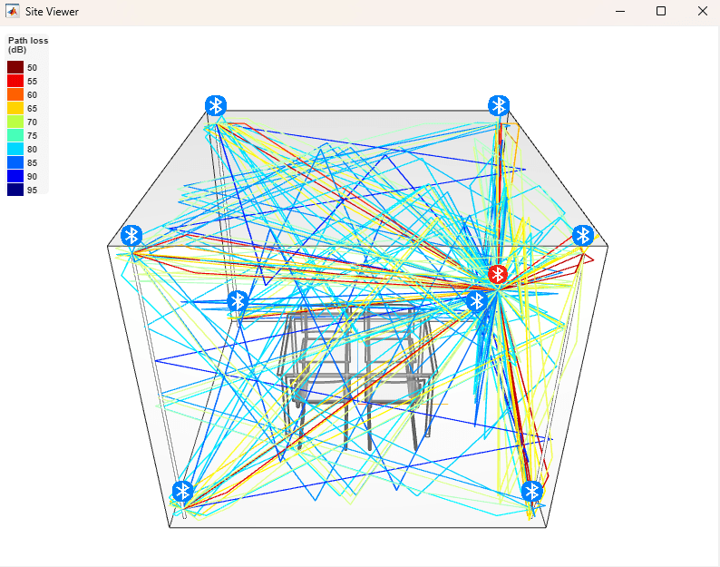

Generate RSSI Fingerprint Features and Labels

Generate RSSIs for each locator-node pair from the received packets by performing this procedure.

The example assumes that locators do not interfere with each other. Each receiver node makes multiple observations to generate the training data. Additionally, before training, you preprocess the RSSI values at each location to rearrange them into a $N_{rssi}$ -by- $N_{locator}$ array. For this example, $N_{rssi}$ is 32 and $N_{locator}$ is 8.

Initialize LE Waveform and Thermal Noise Parameters

To simulate variations in the environment, change the outputPower and noise figure (NF) values. You can change the number of observations collected for each locator-node pair. By increasing numObsPerPair, you can create more data for training.

outputPower = 5;                             % In dBm
noiseFigure = 12;                                                   % In dB
numObsPerPair = 60;
numRSSI = 32;

Each LE locator transmits Bluetooth LE1M or LE2M packets through a noisy channel, and each node receives these packets. The symbol rate for LE1M waveform is 1 Msps, while the LE2M waveform has a symbol rate of 2 Msps. Regardless of the LE PHY mode, the system sets the output waveform to maintain a constant sampling rate of 8 MHz. This is ensured by using an sps of 8 for LE1M waveforms and 4 for LE2M waveforms. The LE packet length is chosen as 256 bits.

packetLength = 256;                                                 
sps = 8;
symbolRate = 1e6;                                                   % In Hz
samplingRate = symbolRate*sps;                                      % In Hz
channelIndex = 38;                                                  % Broadcasting channel index
data = randi([0 1],packetLength,1,"single");
dBdBmConvFactor = 30;
scalingFactor = 10^((outputPower - dBdBmConvFactor)/20);            % dB to linear conversion
txWaveform = cell(2,1);

Generate LE Waveforms

Generate LE1M and LE2M waveform by using the bleWaveformGenerator function. Scale the amplitude of the waveforms based on output power. The generated waveforms have an output power of 5 dBm.

txWaveform{1} = scalingFactor*bleWaveformGenerator(data,ChannelIndex=channelIndex,SamplesPerSymbol=sps);
txWaveform{2} = scalingFactor*bleWaveformGenerator(data,ChannelIndex=channelIndex,SamplesPerSymbol=sps/2,Mode="LE2M");

Create and configure comm.ThermalNoise System object™ to add thermal noise.

thNoise = comm.ThermalNoise(NoiseMethod="Noise figure" ,...
    NoiseFigure=noiseFigure,SampleRate=samplingRate);

Generate RSSI data set

Initialize data set related variables and display statistics.

[numBeacons,numNodes] = size(rays); 
features = zeros(numRSSI,numBeacons,numNodes*numObsPerPair);
labels.position = zeros([numNodes*numObsPerPair 3]);
numDisp = 10;                                                              % Number of display text items shown
delta = (numNodes-1)/(numDisp-1);
progressIdx = [1 floor(delta):floor(delta):numNodes-floor(delta) numNodes];

Between each locator-node pair, generate RSSI values for multiple observations as features. The example trains the CNN by combining RSSI features with labels of the node position.

for nS = 1:numNodes
    for nP = 1:numBeacons
        nC = (nS - 1)*numBeacons + nP;
        if ~isempty(rays{nC})
            wIdx = randi([1 2],1,1);
            txW = txWaveform{wIdx};
            rxData = generateRxData(rays{nC},locators(nP),nodes(nS),txW,numRSSI,samplingRate);
        end
        for nD = 1:numObsPerPair
            if ~isempty(rxData)
                rssiSeq = generateRSSI(rxData,thNoise,numRSSI,dBdBmConvFactor);
                features(:,nP,(nS - 1)*numObsPerPair + nD) = rssiSeq;
            else
                features(:,nP,(nS - 1)*numObsPerPair + nD) = 0;
            end
        end
        release(thNoise);
    end
    labels.class((nS - 1)*numObsPerPair + (1:numObsPerPair)) = categorical(cellstr(nodes(nS).Name));
    labels.position((nS - 1)*numObsPerPair + (1:numObsPerPair),:) = repmat(nodes(nS).AntennaPosition',numObsPerPair,1);    
    if any(nS == progressIdx)
        fprintf("Generating Dataset: %3.2f%% complete.\n", 100*(nS/numNodes))
    end
end

Generating Dataset: 5.56% complete.
Generating Dataset: 11.11% complete.
Generating Dataset: 16.67% complete.
Generating Dataset: 22.22% complete.
Generating Dataset: 27.78% complete.
Generating Dataset: 33.33% complete.
Generating Dataset: 38.89% complete.
Generating Dataset: 44.44% complete.
Generating Dataset: 50.00% complete.
Generating Dataset: 55.56% complete.
Generating Dataset: 61.11% complete.
Generating Dataset: 66.67% complete.
Generating Dataset: 72.22% complete.
Generating Dataset: 77.78% complete.
Generating Dataset: 83.33% complete.
Generating Dataset: 88.89% complete.
Generating Dataset: 94.44% complete.
Generating Dataset: 100.00% complete.

Normalize the RSSI values to fall within the range [0, 1].

for nB = 1:size(features,3)
    features(:,:,nB) = (features(:,:,nB)-min(features(:,:,nB),[],'all'))./(max(features(:,:,nB),[],'all')-min(features(:,:,nB),[],'all'));
end

Neural networks serve as powerful models capable of fitting diverse data sets. To validate the results, you must split the data set into 70% training data, 10% validation data, and 20% test data. Before splitting the data into different sets, shuffle the training data randomly. The training model learns to fit the training data by adjusting its weighted parameters based on the prediction error. The validation data helps you to confirm that the model performs well on the unseen data, and does not overfit the training data.

trainRatio = 0.7;
validationRatio = 0.1;
[training,validation,test] = splitDataSet(features,labels,trainRatio,validationRatio);

Build and Train the Network

This section guides you through the process of building and training a CNN to determine node locations. This figure shows the CNN architecture as defined in [3].

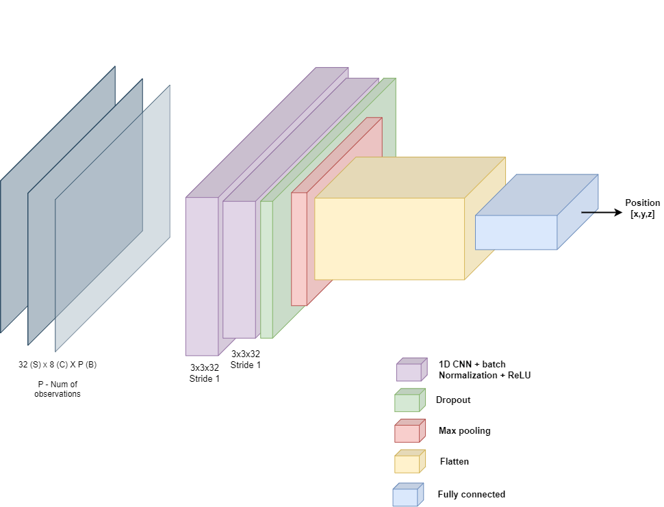
The CNN consists of these components:

Input layer: Defines the size and type of the input data.
Convolutional layer: Performs convolution operations on input to this layer by using a set of filters.
Batch normalization layer: Prevents unstable gradients by normalizing the activations of a layer.
Activation (ReLU) layer: A nonlinear activation function that thresholds the output of the previous functional layer.
Dropout layer: Randomly deactivates a percentage of the parameters of the previous layer during training to prevent overfitting.
Max pooling layer: Performs down sampling by dividing the input into pooling regions and computes maximum of each region.
Flatten layer: Collapses the spatial dimension of the input into its channel dimension.
Output (FC) layer: Defines the size and type of output data. The CNN handles this task as a regression problem.

Construct the CNN.

d = size(features);
layers = [
    
    inputLayer([d(1) d(2) NaN],"SCB")

    convolution1dLayer(3,32,Name="CNN1")
    batchNormalizationLayer
    reluLayer
    
    convolution1dLayer(3,32,Name="CNN1")
    batchNormalizationLayer
    reluLayer
    
    dropoutLayer(0.5)
    maxPooling1dLayer(2,Stride=2)
    
    flattenLayer
    fullyConnectedLayer(3) 
    
    ];

Configure Learning Process and Train the Model

Specify the loss function and training metric. Because the learning process is a regression problem, the example uses minimum square error(MSE) as the loss function. Match the predicted positions to the expected positions for each location. Specify the number of training data samples the model evaluates in each training iteration. If you are working with a larger data set, increase the sample count.

lossFcn = "mse";
trainingMetric = "rmse";

valY = validation.Y;                                             % node actual positions for validation
trainY = training.Y;                                             % node actual positions for training

miniBatchSize = 90; 
validationFrequency = floor(size(training.X,3)/miniBatchSize);

Specify the options that control the training process. The number of epochs determines how many consecutive times the model trains on the full training data set. By default, the model trains on a GPU if available. Training on a GPU requires Parallel Computing Toolbox™ and a supported GPU device. For a list of supported devices, see GPU Computing Requirements (Parallel Computing Toolbox).

options = trainingOptions("adam", ...
    MiniBatchSize=miniBatchSize, ...
    MaxEpochs=5, ...
    InitialLearnRate=1e-3, ...
    ResetInputNormalization=true, ...
    Metrics=trainingMetric, ...
    Shuffle="every-epoch", ...
    ValidationData={validation.X, valY}, ...
    ValidationFrequency=validationFrequency, ...
    ExecutionEnvironment="auto", ...
    Verbose=true);

Train the model.

net = trainnet(training.X,trainY,layers,lossFcn,options);

    Iteration    Epoch    TimeElapsed    LearnRate    TrainingLoss    ValidationLoss    TrainingRMSE    ValidationRMSE
    _________    _____    ___________    _________    ____________    ______________    ____________    ______________
            0        0       00:00:05        0.001                            1.4843                            1.2183
            1        1       00:00:05        0.001          5.3473                            2.3124                  
            8        1       00:00:07        0.001          1.3526            1.2431           1.163             1.115
           16        2       00:00:07        0.001         0.90067           0.80014         0.94904           0.89451
           24        3       00:00:08        0.001         0.72238           0.60449         0.84993           0.77749
           32        4       00:00:08        0.001         0.66188           0.42808         0.81356           0.65428
           40        5       00:00:09        0.001         0.61735           0.26319         0.78572           0.51302
Training stopped: Max epochs completed

Evaluate Model Performance

Predict the node position by passing the test set features through the network.

predPos = minibatchpredict(net,test.X);

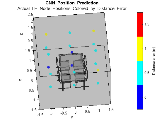
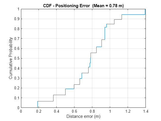
Evaluate the performance of the network by comparing the predicted positions with the expected results. Generate a visual and statistical representation of the results. Assign colors to each LE node for positioning, indicating the distance error of the predicted position from the actual position. The plot displays the actual positions of the LE nodes.

Additionally, generate a cumulative distribution function (CDF), where the y-axis represents the proportion of data with a measured distance error less than or equal to the value on the x-axis. Compute the mean error for all the test predictions from the actual positions.

metric = helperBLEPositioningDLResults(mapFileName,test.Y,predPos);

Figure contains an axes object. The axes object with title CNN blank Position blank Prediction blank Actual LE Node Positions Colored by Distance Error, xlabel x, ylabel y contains 218 objects of type patch, line, scatter.

Figure contains an axes object. The axes object with title CDF - Positioning Error (Mean = 0.81 m), xlabel Distance error (m), ylabel Cumulative Probability contains an object of type stair.

Further Exploration

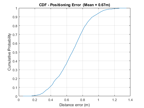
Decreasing the distance between nodes can improve the accuracy of the positioning estimate. If there is no path between the locator and node, packet reception at a location can fail, leading to RSSI values being recorded as 0. When adding more nodes, you must consider those nodes that cannot receive packets from many locators. Collecting RSSI values with more zeros than useful values at some nodes can decrease the accuracy of position estimation. You can increase the maximum number of reflections, or try different transmitter locator placements. Allowing for a higher maximum number of reflections can mitigate scenarios of no packet reception, but at the expense of longer data set generation times. on an Intel(R) Xeon(R) W-2133 CPU @ 3.60 GHz test system in approximately 1 hour and 30 minutes

For example. this plot was generated by using these values.

nodeSeparation = 0.25
numObsPerPair = 200
miniBatchSize = 270
maxEpochs = 20
InitialLearnRate = 1e-4

Appendix

The example uses these helper functions:

helperBLEPositioningDLResults — Visualize indoor location estimation predictions.

References

Bluetooth Technology Website. “Bluetooth Technology Website | The Official Website of Bluetooth Technology.” Accessed May 22, 2024. https://www.bluetooth.com
Bluetooth Special Interest Group (SIG). "Core System Package [Low Energy Controller Volume]". Bluetooth Core Specification. Version 5.3, Volume https://www.bluetooth.com
Shangyi Yang, Chao Sun, and Younguk Kim, "Indoor 3D Localization Scheme Based on BLE Signal Fingerprinting and 1D Convolutional Neural Network", Electronics 10, no. 15 (July 22, 2021): 1758. https://doi.org/10.3390/electronics10151758

Local Functions

function [locators,nodes,antPosNode] = createScenario(nodeSep)
%createScenario Generates the tx locator and rx node objects
%based on separation between the nodes

fc = 2.426e9; % Set the carrier frequency (Hz) to one of broadcasting channels
lambda = physconst("lightspeed")/fc;

txArray = arrayConfig("Size", [1 1], "ElementSpacing", 2*lambda);
rxArray = arrayConfig("Size", [1 1], "ElementSpacing", lambda);


% The dimensions of the room are x:[-1.5 1.5] y:[-1.5 1.5] z:[0 2.5]. 

% Place transmitters at the 8 corners of the room. Choose the x-, y-, 
% and z-coordinates for the locators and generate all possible 
% combinations of x, y, and z from these coordinates.

xLocators = [-1.4 1.4];   % In meters
yLocators = [-1.4 1.4];   % In meters
zLocators = [0.1 2.4];    % In meters

% Define valid space for nodes
xNode = [-1 1];
yNode = [-1 1];
zNode = [0.8 2];

dX = diff(xNode);
dY = diff(yNode);
dZ = diff(zNode);
dims = [dX dY dZ];

% Calculate antenna positions
possC = combinations(xLocators,yLocators,zLocators);
antPosLocator = table2array(possC)';

rxSep = nodeSep;
numSeg = floor(dims/rxSep);
dimsOffset = (dims-(numSeg*rxSep))./2;
xGridNode = (min(xNode)+dimsOffset(1)):rxSep:(max(xNode)-dimsOffset(1));
yGridNode = (min(yNode)+dimsOffset(2)):rxSep:(max(yNode)-dimsOffset(2));
zGridNode = (min(zNode)+dimsOffset(3)):rxSep:(max(zNode)-dimsOffset(3));

% Set the position of the node antenna centroid by replicating the
% position vectors across 3-D space
antPosNode = [repmat(kron(xGridNode, ones(1, length(yGridNode))), 1, length(zGridNode)); ...
    repmat(yGridNode, 1, length(xGridNode)*length(zGridNode)); ...
    kron(zGridNode, ones(1, length(yGridNode)*length(xGridNode)))];

% Create multiple locator and node sites with a single constructor call
locators = txsite("cartesian", ...
    AntennaPosition=antPosLocator, ...
    Antenna=txArray, ...
    TransmitterFrequency=fc);

nodes = rxsite("cartesian", ...
    AntennaPosition=antPosNode, ...
    Antenna=rxArray, ...
    AntennaAngle=[0;90]);

end

function [training,validation,test] = splitDataSet(data,labels,trainRatio,validRatio)
%splitDataSet Create training, validation, and test data by randomly shuffling and splitting the data.

% Generate random indices for training/validation/set splits
[trainInd,valInd,testInd] = dividerand(size(data,3),trainRatio,validRatio,1-trainRatio-validRatio);

% Filter training, validation and test data
trainInd = trainInd(randperm(length(trainInd)));
valInd = valInd(randperm(length(valInd)));
training.X = data(:,:,trainInd);
validation.X = data(:,:,valInd);
test.X = data(:,:,testInd);

% Filter training, validation and test labels
training.Y = labels.position(trainInd,:);
validation.Y = labels.position(valInd,:);
test.Y = labels.position(testInd,:);
end

function rxChan = generateRxData(rays,beacons,nodes,txW,numRSSI,samplingRate)
%generateRxData Initialize Ray tracing channel for specific locator-node
%pair and pass the waveform through the channel
rtChan = comm.RayTracingChannel(rays,beacons,nodes); % Create channel
rtChan.ReceiverVirtualVelocity = [0; 0; 0];          % Stationary Receiver
rtChan.NormalizeImpulseResponses = true;
rtChan.SampleRate = samplingRate;
txWRep = repmat(txW,numRSSI,1);
rxChan = rtChan(txWRep);
end

function rssi = generateRSSI(rxChan,thNoise,numRSSI,dBdBmConvFactor)
%generateRSSI Calculate RSSI values after passing the waveform through
%thermal noise
rxW = thNoise(rxChan);
rxWSplit = reshape(rxW,length(rxW)/numRSSI,numRSSI);
rssiL = mean(abs(rxWSplit).^2);
rssi = 20*log10(rssiL(:))+dBdBmConvFactor; % dbm
end