Predict Battery State of Charge Using LiteRT Block in Simulink
This example shows how to predict the battery state of charge (SOC) by using the LiteRT Block. Battery SOC is the level of charge that an electric battery has relative to its capacity, measured as a percentage. SOC is critical information for vehicle energy management systems and must be accurately estimated to ensure reliable electrified vehicles. Estimating SOC is a challenge in automotive engineering due to the nonlinear behavior of lithium-ion batteries, which is influenced by temperature, battery health, the SOC itself, and other factors. Traditional methods, like electrochemical models, often require detailed knowledge of the composition of the battery and precise physical parameters to estimate the SOC. In neural networks, you can estimate the SOC with minimal prior knowledge about the battery or its nonlinear characteristics.

In this example, you:
Generate C code from a LiteRT model, formally known as a TensorFlow Lite model, and use this code to predict the battery state of charge.
Run the generated code by using the software-in-the-loop (SIL) simulation on the host computer.
Run the generated code by using processor-in-the-loop (PIL) simulation on a Raspberry Pi board.
Network Architecture
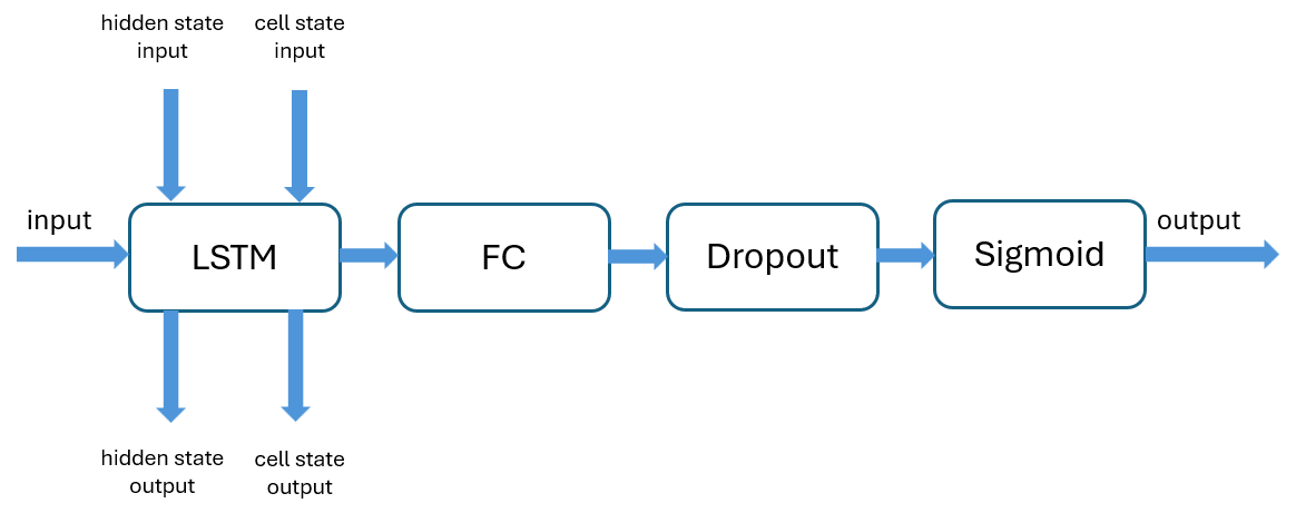
This example uses an LSTM network that can learn long-term trends. It was trained using the LG_HG2_Prepared_Dataset_McMasterUniversity_Jan_2020 data set. The network uses only temperature, voltage, and current from the data set. The network has the following architectures:
LSTM Layer — The network uses this layer with 256 hidden units to learn long-term dependencies in the sequence data. The LSTM layer takes the initial states as inputs and returns the updates states as outputs. The network can update the states by passing the output states as initial states for the next iteration.
Fully Connected Layer — The network uses this layer to match the size of the output.
Dropout Layer — The network uses this layer with a dropout probability of 0.2 to reduce overfitting.
Sigmoid Layer — The network uses this layer to bound the output in the interval
[0,1].
Download Test Data
The downloadTestData helper function downloads the LG_HG2_Prepared_Dataset_McMasterUniversity_Jan_2020 data and the testing data.
[xTrain, yTrain, xVal, yVal, xTest, yTest] = downloadData();
Load Simulink Model
The bsocLiteRTModel model contains two From Workspace blocks that import the model input signal and the ground truth signal. The LiteRT block loads the LSTM network into Simulink®. The LiteRT block outputs the LSTM state outputs from outports out2 and out3 and passes them back to itself as initial states for the next time step by using a feedback loop with a one-step delay. The Scope block displays the model output and the ground truth signal.
modelName = "bsocLiteRTModel";
model = load_system(modelName);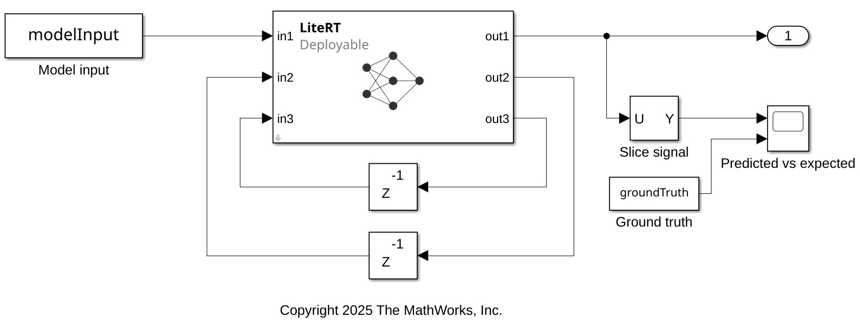
Prepare Inputs and Configure the Simulink Model
Create a variable named sampleTime to control the sample size. Set the stop time of the model.
sampleTime = 1e-4;
numSamples = numel(yTest);
stopTime = (numSamples-1)*sampleTime;
set_param(model, 'StopTime', num2str(stopTime));
Use setProdHwDeviceType helper function to set the product hardware device type.
setProdHwDeviceType(model);
Create input data for the model.
modelInput = timetable(single(xTest'), TimeStep=seconds(sampleTime));
groundTruth = timetable(single(yTest'), TimeStep=seconds(sampleTime));
The observations in xTest are of size 3-by-1, but the model expects an input of size 1-by-1-by-3. To match the expected input size, set the permutation vector for in1 to [3 2 1] for the LiteRT block. This setting transforms the 3-by-1 signal into a 1-by-Inf-by-3 signal.
blockName = "LiteRT";
blockPath = modelName + "/" + blockName;
set_param(blockPath, "InputsTable", ...
    "{'in1','single','[1 inf 3]','[3 2 1]';'in2','single','[1 256]','[1 2]';'in3','single','[1 256]','[1 2]'}")
Generate Code and Run SIL Simulation
Generate code and run the code using SIL simulation mode.
simOut = sim(model, 'SimulationMode', 'Software-in-the-loop (SIL)');
Compare Simulation Output with Ground Truth Signal
Get the predicted battery state of charge from the simulation output.
simOutData = get(simOut,'yout');
YPred = cell2mat(get(simOutData,1).Values.Data);
Compare the predicted battery state of charge produced by the Simulink model with the ground truth signal.
timeSteps = simOut.yout{1}.Values.Time;
plot(timeSteps, YPred, timeSteps, yTest', LineWidth=1.5);
title('Predicted BSOC vs Ground truth')
legend('Predicted BSOC', 'Ground truth', Location='southwest');
grid on;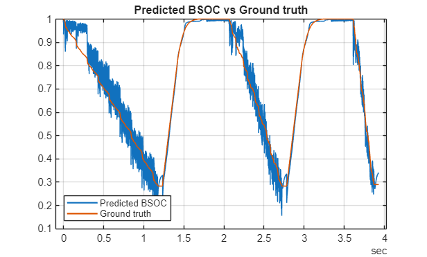
Generate Code and Run PIL Simulation Using Raspberry Pi
Next, deploy the model to hardware. If you have an Embedded Coder® license, you can deploy the model on a hardware. This example uses a Raspberry Pi board. You also need Raspberry Pi® Blockset license to deploy the model to a Raspberry Pi board. For more information, see Raspberry Pi Hardware.
Open the bsocLiteRTModel model.
open_system(modelName);
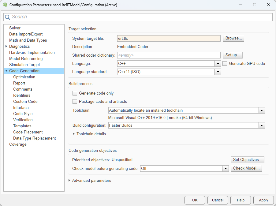
To run the model on a Raspberry Pi board, in the Simulink Toolstrip, click Model Settings to open the Configuration Parameters dialog box. In the Code Generation pane, set System target file to the ert.tlc.
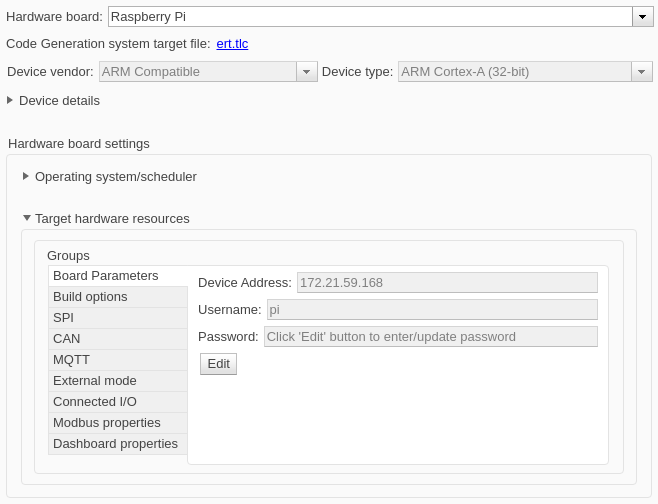
In the Hardware Implementation pane, set Hardware board to Raspberry Pi. Expand the Target hardware resources section and enter the Device Address, Username, and Password parameters for the board.
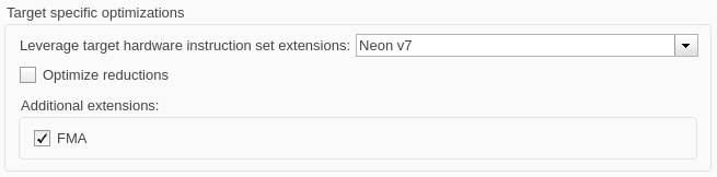
In the Code Generation > Optimization pane, in the Target specific optimizations section, set Leverage target hardware instruction set extensions to Neon v7. To use fast multiply-add to optimize the performance of generated code, select the FMA box. Click OK.
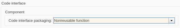
In the Code Generation > Interface pane, set Code interface packing to Nonreusable function, because the Raspberry Pi hardware does not support the default value C++ Class.
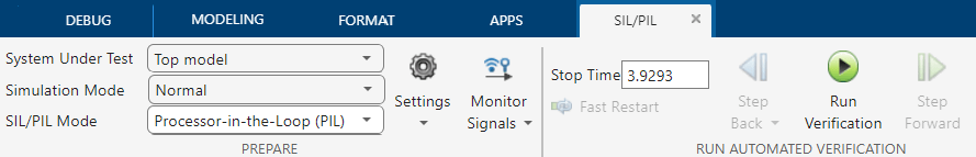
On the Apps tab, click SIL/PIL Manager. In the SIL/PIL tab, in the Mode section, set SIL/PIL Mode to Processor-in-the-Loop (PIL). Then click Run Verification.
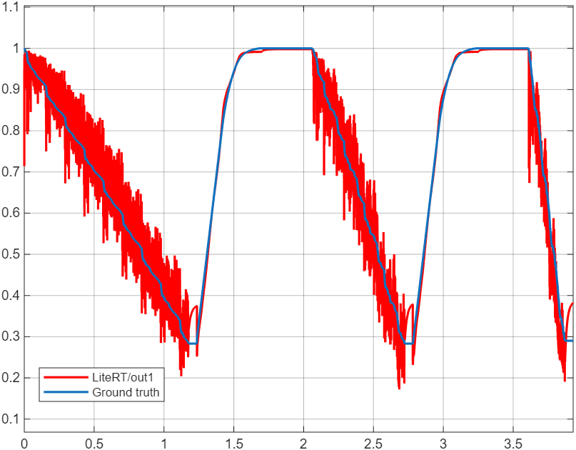
Open the Scope block named Predicted vs expected. The graph displays the predictions of the partially trained LSTM network in red and the expected output in blue.
Helper functions
downloadData
The downloadData function downloads the data for the battery state of charge estimation model.
function [xTrain, yTrain, xVal, yVal, xTest, yTest] = downloadData()

url = "https://data.mendeley.com/public-files/datasets/cp3473x7xv/files/ad7ac5c9-2b9e-458a-a91f-6f3da449bdfb/file_downloaded";
downloadFolder = tempdir;
outputFolder = fullfile(downloadFolder,"LGHG2@n10C_to_25degC");

if ~isfolder(outputFolder)
    disp("Downloading LGHG2@n10C_to_25degC.zip (56 MB) ... ")
    filename = fullfile(downloadFolder,"LGHG2@n10C_to_25degC.zip");
    websave(filename,url);
    unzip(filename,outputFolder)
end

numFeatures = 3;

trainingFile = fullfile(outputFolder,"Train","TRAIN_LGHG2@n10degC_to_25degC_Norm_5Inputs.mat");
[xTrain, yTrain] = setupData(trainingFile,numFeatures);

validationFile = fullfile(outputFolder,"Validation", "01_TEST_LGHG2@n10degC_Norm_(05_Inputs).mat");
[xVal, yVal] = setupData(validationFile,numFeatures);

testFile = fullfile(outputFolder,"Test","01_TEST_LGHG2@n10degC_Norm_(05_Inputs).mat");
s = load(testFile);
xTest = s.X(1:numFeatures,:);
yTest = s.Y;
end

function [x,y] = setupData(filename,numFeatures)
s = load(filename);
x = s.X(1:numFeatures,:)';
y = s.Y';
end
setProdHwDeviceType
The setProdHwDeviceType function sets product hardware device type based on host computer architecture.
function setProdHwDeviceType(model)
if ispc
    prodHWDeviceType = 'Intel->x86-64 (Windows64)';
elseif ismac
    prodHWDeviceType = 'Apple->ARM64';
else
    prodHWDeviceType = 'Intel->x86-64 (Linux 64)';
end
set_param(model, 'ProdHWDeviceType', prodHWDeviceType);
end