compand

This example implements a compander by using a mu-law compressor and expander.

Generate a data sequence.

data = 2:2:12

data = 1×6

     2     4     6     8    10    12

Compress the data sequence by using a mu-law compressor. Set the value for mu to 255. The compressed data sequence now ranges between 8.1 and 12.

compressed = compand(data,255,max(data),'mu/compressor')

compressed = 1×6

    8.1644    9.6394   10.5084   11.1268   11.6071   12.0000

Expand the compressed data sequence by using a mu-law expander. The expanded data sequence is nearly identical to the original data sequence.

expanded = compand(compressed,255,max(data),'mu/expander')

expanded = 1×6

    2.0000    4.0000    6.0000    8.0000   10.0000   12.0000

Calculate the difference between the original data sequence and the expanded sequence.

diffvalue = expanded - data

diffvalue = 1×6
10-14 ×

   -0.0444    0.1776    0.0888    0.1776    0.1776   -0.3553

This example implements a compander by using an A-law compressor and expander.

Generate a data sequence.

data = 1:5;

Compress the data sequence by using an A-law compressor. Set the value for A to 87.6. The compressed data sequence now ranges between 3.5 and 5.

compressed = compand(data,87.6,max(data),'A/compressor')

compressed = 1×5

    3.5296    4.1629    4.5333    4.7961    5.0000

Expand the compressed data sequence by using an A-law expander. The expanded data sequence is nearly identical to the original data sequence.

expanded = compand(compressed,87.6,max(data),'A/expander')

expanded = 1×5

    1.0000    2.0000    3.0000    4.0000    5.0000

Calculate the difference between the original data sequence and the expanded sequence.

diffvalue = expanded - data

diffvalue = 1×5
10-14 ×

         0         0    0.1332    0.0888    0.0888

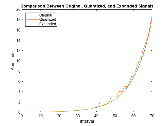
When transmitting signals with a high dynamic range, quantization using equal length intervals can result in signal distortion and a loss of precision. Companding applies a logarithmic computation to compress the signal before quantization on the transmit side and to expand the signal to restore it to full scale on the receive side. Companding avoids signal distortion without the need to specify many quantization levels. Compare distortion when using 6-bit quantization on an exponential signal with and without companding. Plot the original exponential signal, the quantized signal, and the expanded signal.

Create an exponential signal and calculate its maximum value.

sig = exp(-4:0.1:4);
V = max(sig);

Quantize the signal by using equal-length intervals. Set partition and codebook values, assuming 6-bit quantization. Calculate the mean square distortion.

partition = 0:2^6 - 1;
codebook = 0:2^6;
[~,qsig,distortion] = quantiz(sig,partition,codebook);

Compress the signal by using the compand function configured to apply the mu-law method. Apply quantization and expand the quantized signal. Calculate the mean square distortion of the companded signal.

mu = 255; % mu-law parameter
csig_compressed = compand(sig,mu,V,'mu/compressor');
[~,quants] = quantiz(csig_compressed,partition,codebook);
csig_expanded = compand(quants,mu,max(quants),'mu/expander');
distortion2 = sum((csig_expanded - sig).^2)/length(sig);

Compare the mean square distortion for quantization versus combined companding and quantization. The distortion for the companded and quantized signal is an order of magnitude lower than the distortion of the quantized signal. Equal-length intervals are well suited to the logarithm of an exponential signal but not well suited to an exponential signal itself.

[distortion, distortion2]

ans = 1×2

    0.5348    0.0397

Plot the original exponential signal, the quantized signal, and the expanded signal. Zoom in on the axis to highlight the quantized signal error at lower signal levels.

plot([sig' qsig' csig_expanded']);
title('Comparison of Original, Quantized, and Expanded Signals');
xlabel('Interval');
ylabel('Apmlitude');
legend('Original','Quantized','Expanded','location','nw');
axis([0 70 0 20])