Represent Partitions

A quantization partition defines several contiguous, nonoverlapping ranges of values within a set of real numbers. To specify a partition, list the distinct endpoints of the different ranges in a vector.

For example, suppose the partition separates the real number line into the four sets or intervals:

Then you can represent the partition as a three-element vector:

partition = [0,1,3];

The length of the partition vector is one less than the number of partition intervals.

Represent Codebooks

A codebook tells the quantizer which common value to assign to inputs that fall into the distinct intervals defined by the partition vector. Represent a codebook as a vector whose length is the same as the number of partition intervals. For example:

codebook = [-1, 0.5, 2, 3];

This vector is one possible codebook for the partition vector [0,1,3].

Determine Quantization Interval for Each Input Sample

To determine quantization intervals, in this example, you examine the index and quants vectors returned by the quantiz function. The index vector indicates the quantization interval for each input sample as specified by the input partition vector and the quants vector maps the input samples to quantization values specified by the input codebook vector.

Quantize a set of data by using the quantiz function with the specified partition and examine the returned vector index. If you run quantiz without specifying a codebook input, the function assigns the codebook quantization values based on the partition values.

data = [2 9 8];
partition = [3,4,5,6,7,8,9];
index = quantiz(data,partition)

index = 1×3

     0     6     5

The index vector that indicates the input data samples, [2 9 8], lie within the intervals labeled 0, 6, and 5 because partition specifies that

Suppose you continue this example by defining a codebook vector as follows:

codebook = [3,3,4,5,6,7,8,9];

Then this formula relates the vector index to the quantized signal quants.

quants = codebook(index+1)

quants = 1×3

     3     8     7

This formula for quants is exactly what the quantiz function uses if you input the codebook vector and return the quants vector. Examine the returned vector quants to see the partition vector intervals [0 6 5] map to the quantization values [3 8 7] as defined by the codebook vector.

partition = [3,4,5,6,7,8,9];
codebook = [3,3,4,5,6,7,8,9];
[index,quants] = quantiz(data,partition,codebook)

index = 1×3

     0     6     5

quants = 1×3

     3     8     7

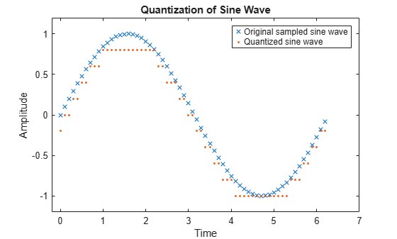
Quantize Sampled Sine Wave

To illustrate the nature of scalar quantization, this example shows how to quantize a sine wave. Plot the original and quantized signals to contrast the x symbols that make up the sine curve with the dots that make up the quantized signal. The vertical coordinate of each dot is a value in the vector codebook.

Generate a sine wave sampled at times defined by t. Specify the partition input by defining the distinct endpoints of the different intervals as the element values of the vector. Specify the codebook input with an element value for each interval defined in the partition vector. The codebook vector must be one element longer than the partition vector.

t = [0:.1:2*pi];
sig = sin(t);
partition = [-1:.2:1];
codebook = [-1.2:.2:1];

Perform quantization on the sampled sine wave.

[index,quants] = quantiz(sig,partition,codebook);

Plot the quantized sine wave and the sampled sine wave.

plot(t,sig,'x',t,quants,'.')
title('Quantization of Sine Wave')
xlabel('Time')
ylabel('Amplitude')
legend('Original sampled sine wave','Quantized sine wave');
axis([-.2 7 -1.2 1.2])

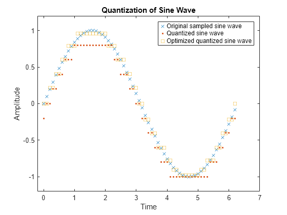
Optimize Quantization Parameters

Testing and selecting parameters for large signal sets with a fine quantization scheme can be tedious. One way to produce partition and codebook parameters easily is to optimize them according to a set of training data. The training data should be typical of the kinds of signals to be quantized.

This example uses the lloyds function to optimize the partition and codebook according to the Lloyd algorithm. The code optimizes the partition and codebook for one period of a sinusoidal signal, starting from a rough initial guess. Then the example runs the quantiz function twice to generate quantized data by using the initial partition and codebook input values and by using the optimized partitionOpt and codebookOpt input values. The example also compares the distortion for the initial and the optimized quantization.

Define variables for a sine wave signal and initial quantization parameters. Optimize the partition and codebook by using the lloyds function.

t = 0:.1:2*pi;
sig = sin(t);
partition = -1:.2:1;
codebook = -1.2:.2:1;
[partitionOpt,codebookOpt] = lloyds(sig,codebook);

Generate quantized signals by using the initial and the optimized partition and codebook vectors. The quantiz function automatically computes the mean square distortion and returns it as the third output argument. Compare mean square distortions for quantization with the initial and optimized input arguments to see how less distortion occurs when using the optimized quantized values.

[index,quants,distor] = quantiz(sig,partition,codebook);
[indexOpt,quantOpt,distorOpt] = ...
    quantiz(sig,partitionOpt,codebookOpt);
[distor, distorOpt]

ans = 1×2

    0.0148    0.0022

Plot the sampled sine wave, the quantized sine wave, and the optimized quantized sine wave.

plot(t,sig,'x',t,quants,'.',t,quantOpt,'s')
title('Quantization of Sine Wave')
xlabel('Time')
ylabel('Amplitude')
legend('Original sampled sine wave', ...
    'Quantized sine wave', ...
    'Optimized quantized sine wave');
axis([-.2 7 -1.2 1.2])

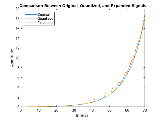
Quantize and Compand an Exponential Signal

When transmitting signals with a high dynamic range, quantization using equal length intervals can result in signal distortion and a loss of precision. Companding applies a logarithmic computation to compress the signal before quantization on the transmit side and to expand the signal to restore it to full scale on the receive side. Companding avoids signal distortion without the need to specify many quantization levels. Compare distortion when using 6-bit quantization on an exponential signal with and without companding. Plot the original exponential signal, the quantized signal, and the expanded signal.

Create an exponential signal and calculate its maximum value.

sig = exp(-4:0.1:4);
V = max(sig);

Quantize the signal by using equal-length intervals. Set partition and codebook values, assuming 6-bit quantization. Calculate the mean square distortion.

partition = 0:2^6 - 1;
codebook = 0:2^6;
[~,qsig,distortion] = quantiz(sig,partition,codebook);

Compress the signal by using the compand function configured to apply the mu-law method. Apply quantization and expand the quantized signal. Calculate the mean square distortion of the companded signal.

mu = 255; % mu-law parameter
csig_compressed = compand(sig,mu,V,'mu/compressor');
[~,quants] = quantiz(csig_compressed,partition,codebook);
csig_expanded = compand(quants,mu,max(quants),'mu/expander');
distortion2 = sum((csig_expanded - sig).^2)/length(sig);

Compare the mean square distortion for quantization versus combined companding and quantization. The distortion for the companded and quantized signal is an order of magnitude lower than the distortion of the quantized signal. Equal-length intervals are well suited to the logarithm of an exponential signal but not well suited to an exponential signal itself.

[distortion, distortion2]

ans = 1×2

    0.5348    0.0397

Plot the original exponential signal, the quantized signal, and the expanded signal. Zoom in on the axis to highlight the quantized signal error at lower signal levels.

plot([sig' qsig' csig_expanded']);
title('Comparison of Original, Quantized, and Expanded Signals');
xlabel('Interval');
ylabel('Apmlitude');
legend('Original','Quantized','Expanded','location','nw');
axis([0 70 0 20])