Visualize Coverage Maps over Lunar Terrain Using Ray Tracing
Display viewsheds and coverage maps for a base station on the surface of the Moon using terrain data and ray tracing analysis. A viewshed includes areas that are within line of sight (LOS) of a set of points, and a coverage map includes received power for the areas within range of a set of wireless transmitters. You can use a viewshed as a first-order approximation of a coverage map.
The goal of this example is to analyze radio coverage for a lunar module during several extra-vehicular activities (EVAs). During these EVAs, a moon rover travels from the lunar module to nearby hill clusters. The trajectories of the moon rover are based on the 1971 Apollo 15 mission, which was the first Apollo mission to use a moon rover. Because the moon rover enabled EVAs of longer distances than previous Apollo missions, maintaining communications between the rover, the module, and Earth was critical to the mission. During the mission, the rover frequently drove through areas with no radio coverage, inhibiting communication with the module.
When using geographic coordinates, the ray tracing capabilities in Antenna Toolbox™ and Communications Toolbox™ use an Earth-based area of interest (AOI). By combining the ray tracing capabilities with the mapping capabilities in Mapping Toolbox™, you can visualize coverage over generic planetary terrain.
This example shows you how to:
Read lunar terrain data and a reference spheroid from a GeoTIFF file.
Get a reference ellipsoid for the Moon.
Generate the trajectory of a moon rover.
View terrain, coverage maps, and viewsheds in 2-D.
View terrain and propagation paths in 3-D.
Read Terrain and Reference Spheroid
Read terrain elevation data for the AOI and a reference spheroid for the moon. The reference spheroid enables you to generate the trajectory of the moon rover, to perform the ray tracing analysis, and to create maps of the region.
The Apollo 15 mission took place in a region surrounding the Hadley Plains. Read lunar terrain elevation data [1] for the Hadley Plains from a GeoTIFF file. The file reports elevations in meters with respect to a reference spheroid that represents the shape of the Moon. You can download the data in JPEG 2000 format from the Goddard Space Flight Center [2]. The file used in this example has been cropped from the original data set and exported to a GeoTIFF file.
filename = "SLDEM2015_Hadley_Plains_Apollo15.tif";
[Z,R] = readgeoraster(filename,OutputType="double");
The readgeoraster function imports the data into the workspace as an array and a raster reference object in geographic coordinates. The reference object stores information such as the latitude limits, the longitude limits, and the geographic coordinate reference system (CRS). Display the properties of the reference object.
disp(R)
  GeographicCellsReference with properties:

             LatitudeLimits: [24.6328125 27.630859375]
            LongitudeLimits: [2.134765625 5.1328125]
                 RasterSize: [307 307]
       RasterInterpretation: 'cells'
           ColumnsStartFrom: 'north'
              RowsStartFrom: 'west'
       CellExtentInLatitude: 0.009765625
      CellExtentInLongitude: 0.009765625
     RasterExtentInLatitude: 2.998046875
    RasterExtentInLongitude: 2.998046875
           XIntrinsicLimits: [0.5 307.5]
           YIntrinsicLimits: [0.5 307.5]
       CoordinateSystemType: 'geographic'
              GeographicCRS: [1×1 geocrs]
                  AngleUnit: 'degree'
The geographic CRS stores the reference spheroid for the Moon. Extract the reference spheroid from the CRS.
moonSpheroid = R.GeographicCRS.Spheroid;
Define Lunar Module, Moon Rover, and Trajectory of Rover
Specify the latitude and longitude coordinates [3] of the lunar module. Approximate the height of the lunar module in meters.
moduleLat = 26.132;
moduleLon = 3.634;
moduleHeight = 7;
The lunar module uses the Unified-S band radio system for tracking and communication. Specify the frequency in hertz and the power in watts [4].
moduleFreq = 2.82e9;
modulePower = 20;
Approximate the height of the moon rover in meters.
roverHeight = 1.5;
Approximate the trajectories of three EVAs: one to the Hadley Rille, another to the Mons Hadley Delta hill complex, and the last to the South Cluster hill complex. For each trajectory:
Specify the approximate coordinates of the rover destination.
Calculate the trajectory by finding the coordinates of points between the lunar module and the rover destination. Get points along a geodesic on the Moon by using the
track2function and specifying the Moon reference spheroid.
% trajectory to Hadley Rille
eva1Lat = 26.15;
eva1Lon = 3.56;
[traj1Lat,traj1Lon] = track2(moduleLat,moduleLon,eva1Lat,eva1Lon,moonSpheroid);

% trajectory to Mons Hadley Delta hill complex
eva2Lat = 26.01;
eva2Lon = 3.59;
[traj2Lat,traj2Lon] = track2(moduleLat,moduleLon,eva2Lat,eva2Lon,moonSpheroid);

% trajectory to South Cluster hill complex
eva3Lat = 25.98;
eva3Lon = 3.697;
[traj3Lat,traj3Lon] = track2(moduleLat,moduleLon,eva3Lat,eva3Lon,moonSpheroid);
To facilitate plotting, collect the rover destination and trajectory variables for each EVA into combined variables. Use one variable each for these attributes: destination latitudes, destination longitudes, destination heights, trajectory latitudes, trajectory longitudes, and trajectory heights.
evaLat = [eva1Lat; eva2Lat; eva3Lat];
evaLon = [eva1Lon; eva2Lon; eva3Lon];
evaHeight = ones(length(evaLat),1) * roverHeight;

trajLat = [traj1Lat; traj2Lat; traj3Lat];
trajLon = [traj1Lon; traj2Lon; traj3Lon];
trajHeight = ones(length(trajLat),1) * roverHeight;
Specify the colors to use when plotting the trajectories, the lunar module, and the rover destinations. Use white for the trajectories, red for the lunar module, yellow for the rover destinations, and black for the marker outlines.
trajColor = "w";
moduleColor = "r";
roverColor = "y";
outlineColor = "k";
Visualize Terrain and Viewshed in 2-D
Visualize the terrain for the region and the viewshed from the lunar module by using map axes. Map axes enable you to display geographic data using a map projection.
Visualize Terrain
Visualize the terrain for the region.
Set up a map axes object for the region by using the setUpMapAxes helper function. The function creates the map from a projected CRS and the limits stored in a raster reference object. Specify the CRS using the Moon 2000 Equidistant Cylindrical projected CRS, which has the ESRI authority code 103881. The equidistant cylindrical projection is a reasonable choice for the region because it minimizes distortion near the equator.
figure
moonProjectedCRS = projcrs(103881,Authority="ESRI");
setUpMapAxes(moonProjectedCRS,R)
Display the terrain data on the map using a pseudocolor raster plot, which applies color using the colormap of the axes. Add a labeled color bar.
geopcolor(Z,R)

cb = colorbar;
cb.Label.String = "Elevation in meters (with respect to reference spheroid)";
Display the trajectories on the map using white lines.
geoplot(trajLat,trajLon,Color=trajColor)
Display the lunar module on the map using a red circle marker. Prepare to include the module in a legend by specifying a display name and setting the plot object to a variable.
modulePt = geoscatter(moduleLat,moduleLon, ...
    Marker="o",SizeData=50,MarkerFaceColor=moduleColor, ...
    LineWidth=1.2,MarkerEdgeColor=outlineColor, ...
    DisplayName="Lunar Module");
Display the rover destinations on the map using yellow triangle markers. Prepare to include the destinations in the legend by specifying a display name and setting the plot object to a variable.
roverPt = geoscatter(evaLat,evaLon, ...
    Marker="^",SizeData=50,MarkerFaceColor=roverColor, ...
    LineWidth=1.2,MarkerEdgeColor=outlineColor, ...
    DisplayName="Rover Destination");
Add a title. Include the lunar module and the rover destinations in a legend.
title("Lunar Terrain for Hadley Plains")
legend([modulePt roverPt])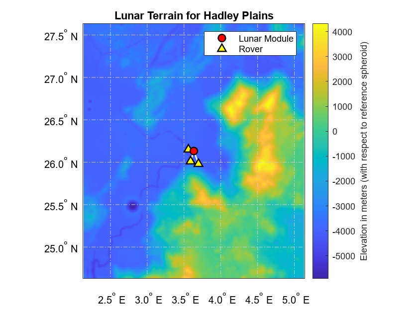
Visualize Terrain for AOI
Visualize the terrain for only the area surrounding the lunar module by resampling the terrain data to a smaller region.
Specify an AOI by finding the coordinates of points that are 5 kilometers north, east, south, and west of the lunar module. Calculate the latitude and longitude limits of the AOI.
[boundinglat,boundinglon] = reckon(moduleLat,moduleLon,5000,[0; 90; 180; 270],moonSpheroid);
AOI = aoiquad(boundinglat,boundinglon);
[latlim,lonlim] = bounds(AOI);
Create a reference object for the AOI by making a copy of the original reference object and changing the latitude and longitude limits. Specify a new raster size of 200 rows and 200 columns. Then, resample the terrain elevation data.
RAOI = R;
RAOI.LatitudeLimits = latlim;
RAOI.LongitudeLimits = lonlim;

gridSize = [200 200];
RAOI.RasterSize = gridSize;

ZAOI = georesample(Z,R,RAOI,"cubic");
Set up a new map. Display the terrain data on the map and add a labeled color bar.
figure
setUpMapAxes(moonProjectedCRS,RAOI)

geopcolor(ZAOI,RAOI)

cb = colorbar;
cb.Label.String = "Elevation in meters (with respect to reference spheroid)";
Display the trajectories, the lunar module, and the rover destinations on the map.
geoplot(trajLat,trajLon,Color=trajColor,LineWidth=1.5)

modulePt = geoscatter(moduleLat,moduleLon, ...
    Marker="o",SizeData=150,MarkerFaceColor=moduleColor, ...
    LineWidth=1.2,MarkerEdgeColor=outlineColor, ...
    DisplayName="Lunar Module");

roverPt = geoscatter(evaLat,evaLon, ...
    Marker="^",SizeData=150,MarkerFaceColor=roverColor, ...
    LineWidth=1.2,MarkerEdgeColor=outlineColor, ...
    DisplayName="Rover Destination");
Add a title. Include the lunar module and the rover destinations in a legend.
legend([modulePt roverPt])
title("Lunar Terrain for AOI")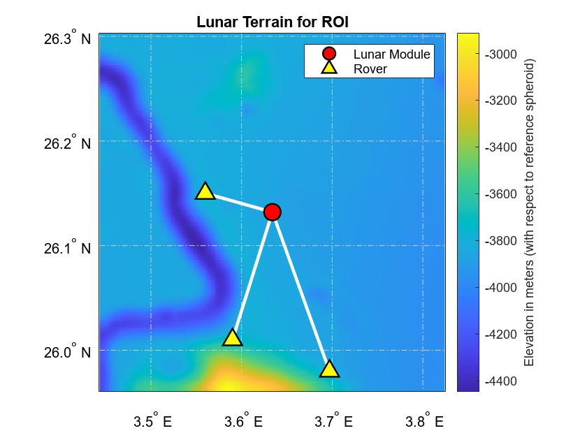
Visualize Viewshed for AOI
Calculate the viewshed for the lunar module. Indicate that the heights of the lunar module and the grid coordinates are referenced to the terrain by specifying the height references as "AGL". Specify the radius of the reference sphere using the Moon spheroid.
visBase = viewshed(ZAOI,RAOI,moduleLat,moduleLon, ...
    moduleHeight,roverHeight,"AGL","AGL",moonSpheroid.Radius);
The visBase array returned by the viewshed function indicates visible areas using values of 1 and obscured areas using values of 0. To avoid plotting the obscured areas, replace the 0 values with NaN values. Define a colormap for the viewshed that uses turquoise for visible areas.
visBase(visBase == 0) = NaN;
covcolor = [0.1034  0.8960  0.7150];
Set up a new map. Provide geographic context for the viewshed by displaying the terrain data as a grayscale image.
figure
setUpMapAxes(moonProjectedCRS,RAOI)

grayZAOI = rescale(ZAOI);
geoimage(grayZAOI,RAOI)
Display the viewshed over the terrain data by using a pseudocolor raster plot and the viewshed colormap. Prepare to include the viewshed in a legend by specifying a display name and setting the plot object to a variable.
viewshedPlot = geopcolor(visBase,RAOI,DisplayName="Viewshed");
colormap(covcolor)
Display the trajectories, the lunar module, and the rover destinations on the map.
geoplot(trajLat,trajLon,Color=trajColor,LineWidth=1.5)

modulePt = geoscatter(moduleLat,moduleLon, ...
    Marker="o",SizeData=150,MarkerFaceColor=moduleColor, ...
    LineWidth=1.2,MarkerEdgeColor=outlineColor, ...
    DisplayName="Lunar Module");

roverPt = geoscatter(evaLat,evaLon, ...
    Marker="^",SizeData=150,MarkerFaceColor=roverColor, ...
    LineWidth=1.2,MarkerEdgeColor=outlineColor, ...
    DisplayName="Rover Destination");
Add a title. Include the viewshed, the lunar module, and the rover destinations in a legend.
legend([viewshedPlot modulePt roverPt])
title("Viewshed of Apollo 15 Lunar Module")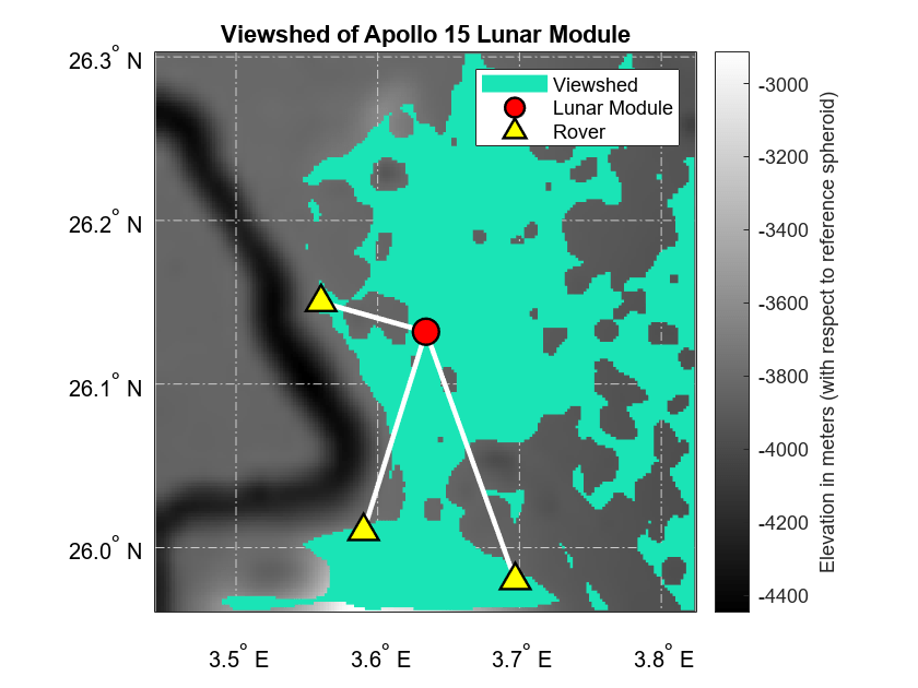
Visualize Coverage in 2-D
A viewshed is comparable to a coverage map that includes only line-of-sight (LOS) propagation. You can create more detailed coverage maps and calculate received power by using antenna sites and ray tracing propagation models.
Create Antenna Sites
Prepare to create a coverage map by creating a transmitter site for the base station and a grid of receiver sites for the AOI.
To use a ray tracing propagation model with imported elevation data, you must specify the locations of the antenna sites using Cartesian coordinates. You can transform geographic coordinates to Cartesian coordinates in a local ENU system by using the helperLatLonToENU helper function.
Create Transmitter Site
Specify the local origin of the ENU coordinate system using the geographic coordinates of the lunar module.
originlat = moduleLat;
originlon = moduleLon;
originht = 0;
Specify the geographic coordinates of the transmitter site. Then, transform the geographic coordinates to ENU coordinates by using the helperLatLonToENU helper function.
txlat = moduleLat;
txlon = moduleLon;
[txx,txy,txz] = helperLatLonToENU(Z,R,txlat,txlon,originlat,originlon,0,moonSpheroid);
Place the base station on top of the lunar module by adjusting the ENU z-coordinate.
txz = txz + moduleHeight;
Create the transmitter site. By default, transmitter sites use isotropic antennas.
tx = txsite("cartesian", ...
    AntennaPosition=[txx; txy; txz], ...
    TransmitterFrequency=moduleFreq, ...
    TransmitterPower=modulePower);
Create Receiver Sites
Extract a grid of geographic coordinates from the reference object for the AOI. Then, transform the geographic coordinates to local ENU coordinates by using the helperLatLonToENU helper function.
[latAOI,lonAOI] = geographicGrid(RAOI);
[rxx,rxy,rxz] = helperLatLonToENU(Z,R,latAOI(:),lonAOI(:), ...
    originlat,originlon,originht,moonSpheroid);
Place the receiver sites above the moon rover by adjusting the ENU z-coordinates.
rxz = rxz + roverHeight;
Create the receiver sites.
rxs = rxsite("cartesian",AntennaPosition=[rxx rxy rxz]');Create Triangulation of Lunar Surface
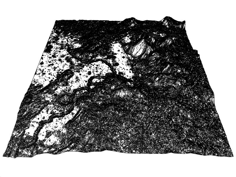
Convert the terrain elevation data to a triangulation object. A triangulation object enables you to create coverage maps using ray tracing propagation model objects.
To use the ray tracing propagation model with a triangulation object, you must use a triangulation object referenced to Cartesian coordinates. Extract a grid of geographic coordinates from the reference object for the terrain data.
[gridlat,gridlon] = geographicGrid(R);
Convert the coordinates to Cartesian coordinates in an east-north-up (ENU) local coordinate system. Specify the origin of the ENU system using the coordinates of the lunar module.
[x,y,z] = geodetic2enu(gridlat,gridlon,Z,originlat,originlon,originht,moonSpheroid);
Convert the Cartesian coordinates to a patch with triangular faces. The surf2patch function represents the patch using two variables: V contains the patch vertices, and F determines which vertices to connect to form each triangular face. Prepare to visualize the triangulation object by reordering the vertices. Then, create the triangulation object from the patch.
[F,V] = surf2patch(x,y,z,"triangles");
F = F(:,[1 3 2]);
tri = triangulation(F,V);
Create Ray Tracing Propagation Model
Create a ray tracing propagation model, which MATLAB® represents using a RayTracing object. Specify the surface material using the real relative permittivity and the conductivity of the Moon surface [5]. By default, the model uses the shooting-and-bouncing rays (SBR) method.
epsR = 3.7;                                    % real relative permittivity of Moon surface
lossTan = 0.1;                                 % dielectric loss tangent
epsilon = 8.8541878128e-12;                    % permittivity of free space (vacuum)
cond = lossTan*(2*pi*moduleFreq)*epsR*epsilon; % conductivity of Moon surface

pm = propagationModel("raytracing",CoordinateSystem="cartesian", ...
    SurfaceMaterial="custom",SurfaceMaterialPermittivity=epsR, ...
    SurfaceMaterialConductivity=cond);
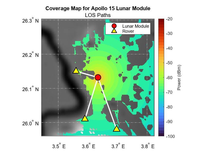
Visualize Line-of-Sight Coverage
Configure the propagation model to find LOS paths. Then, calculate the received power, in dBm, at each receiver site. Specify the terrain using the triangulation object.
pm.MaxNumReflections = 0;
sslos = sigstrength(rxs,tx,pm,Map=tri);
Prepare to display the coverage map.
Specify power levels of interest between –120 dBm and –50 dBm.
Define a colormap that uses 5 colors per 10 dBm.
Specify colormap limits.
Reshape the power values into a grid, and replace values below the minimum power threshold with
NaNvalues.
levels = -120:10:-50;
cmap = turbo(5*length(levels));
climLevels = [min(levels)+20 max(levels)+30];

ss = sslos;
ss = reshape(ss,gridSize);
ss (ss < min(levels)) = NaN;
Set up a new map. Provide geographic context for the coverage map by displaying the terrain data as a grayscale image.
figure
setUpMapAxes(moonProjectedCRS,RAOI)
geoimage(grayZAOI,RAOI)
Display the received power values using a pseudocolor raster plot. Apply the power level colormap and set the color limits. Add a labeled color bar.
geopcolor(ss,RAOI)

colormap(cmap)
clim(climLevels)

cb = colorbar;
cb.Label.String = "Power (dBm)";
Display the trajectories, the lunar module, and the rover destinations in the second map.
geoplot(trajLat,trajLon,Color=trajColor,LineWidth=1.5)

modulePt = geoscatter(moduleLat,moduleLon, ...
    Marker="o",SizeData=150,MarkerFaceColor=moduleColor, ...
    LineWidth=1.2,MarkerEdgeColor=outlineColor, ...
    DisplayName="Lunar Module");

roverPt = geoscatter(evaLat,evaLon, ...
    Marker="^",SizeData=150,MarkerFaceColor=roverColor, ...
    LineWidth=1.2,MarkerEdgeColor=outlineColor, ...
    DisplayName="Rover Destination");
Add a title and subtitle. Include the lunar module and the rover destinations in a legend.
title("Coverage Map for Apollo 15 Lunar Module")
subtitle("LOS Paths")
legend([modulePt roverPt])
Visualize Coverage with One Reflection
Configure the propagation model to find paths with up to one surface reflection. Then, recalculate the received power, in dBm, at each receiver site.
pm.MaxNumReflections = 1;
ssref = sigstrength(rxs,tx,pm,Map=tri);
Prepare to display the coverage map by reshaping the power values into a grid and by replacing values below the minimum threshold with NaN values.
ss = ssref;
ss = reshape(ss,gridSize);
ss (ss < min(levels)) = NaN;
Set up a new map. Provide geographic context for the coverage map by displaying the terrain data as a grayscale image.
figure
setUpMapAxes(moonProjectedCRS,RAOI)
geoimage(grayZAOI,RAOI)
Display the received power values using a pseudocolor raster plot. Apply the power level colormap and set the color limits. Add a labeled color bar.
geopcolor(ss,RAOI)

colormap(cmap)
clim(climLevels)

cb = colorbar;
cb.Label.String = "Power (dBm)";
Display the trajectories, the lunar module, and the rover destinations in the second tile.
geoplot(trajLat,trajLon,Color=trajColor,LineWidth=1.5)

modulePt = geoscatter(moduleLat,moduleLon, ...
    Marker="o",SizeData=150,MarkerFaceColor=moduleColor, ...
    LineWidth=1.2,MarkerEdgeColor=outlineColor, ...
    DisplayName="Lunar Module");

roverPt = geoscatter(evaLat,evaLon, ...
    Marker="^",SizeData=150,MarkerFaceColor=roverColor, ...
    LineWidth=1.2,MarkerEdgeColor=outlineColor, ...
    DisplayName="Rover Destination");
Add a title and subtitle. Include the lunar module and the rover destinations in a legend.
title("Coverage Map for Apollo 15 Lunar Module")
subtitle("LOS Paths and Paths with 1 Reflection")
legend([modulePt roverPt])

While the addition of paths with one reflection does not change the general shape of the coverage area, the interference between the line-of-sight paths and the reflected paths cause speckles in the power profile.
Visualize Terrain and Propagation Paths in 3-D
Visualize the terrain and propagation paths in 3-D using Site Viewer.
Import the triangulation object that represents the terrain model into Site Viewer. View the terrain for the AOI by zooming out and rotating the model.
sv = siteviewer(SceneModel=tri,ShowEdges=false,ShowOrigin=false);
Create a receiver site that represents the destination for the EVA to the Mons Hadley Delta hill complex. Convert the geographic coordinates to local ENU coordinates by using the helperLatLonToENU function.
[rxx,rxy,rxz] = helperLatLonToENU(Z,R,eva2Lat,eva2Lon, ...
    originlat,originlon,originht,moonSpheroid);
rxz = rxz + roverHeight;
rx = rxsite("cartesian",AntennaPosition=[rxx rxy rxz]');
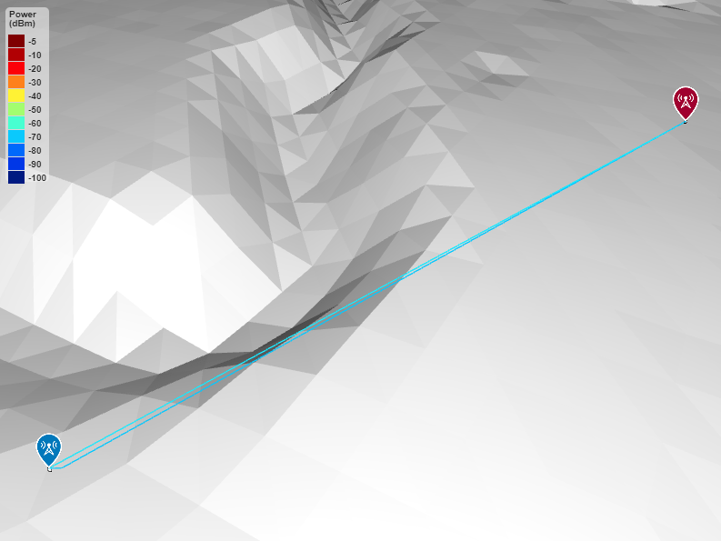
Display the transmitter site, the receiver site, and the LOS visibility status from the lunar module to the rover destination. The green line indicates that the rover is within LOS of the lunar module.
show(tx)
show(rx)
los(tx,rx)

Calculate and display the LOS and single-reflection propagation paths between transmitter and the receiver.
raytrace(tx,rx,pm,ColorLimits=[-100 -5])
References
[1] Barker, M.K., E. Mazarico, G.A. Neumann, M.T. Zuber, J. Haruyama, and D.E. Smith. "A New Lunar Digital Elevation Model from the Lunar Orbiter Laser Altimeter and SELENE Terrain Camera." Icarus 273 (July 2016): 346–55. https://doi.org/10.1016/j.icarus.2015.07.039.
[2] NASA's Planetary Geology, Geophysics and Geochemistry Laboratory. "PGDA - High-resolution Lunar Topography (SLDEM2015)." NASA Goddard Space Flight Center. Accessed August 28, 2023. https://pgda.gsfc.nasa.gov/products/54.
[3] Davies, Merton E., and Tim R. Colvin. "Lunar Coordinates in the regions of the Apollo landers." Journal of Geophysical Research: Planets 105, no. E8 (2000): 20277–80. https://doi.org/10.1029/1999JE001165.
[4] Peltzer, K.E. “Apollo Unified S-Band System.” Technical Memorandum (TM). Greenbelt, Maryland: NASA Goddard Space Flight Center, April 1, 1966. https://ntrs.nasa.gov/citations/19660018739.
[5] Heiken, Grant, David Vaniman, and Bevan M. French, eds. Lunar Sourcebook: A User’s Guide to the Moon. Cambridge [England]; New York: Cambridge University Press, 1991.
Helper Functions
The setUpMapAxes function sets up a map axes object for a region using the projected CRS pcrs and the geographic raster reference object geoR. Within the function:
Create a map axes object using the projected CRS. Set the hold state of the axes to
"on".Apply a cartographic map layout.
Set the cartographic limits using the latitude and longitude limits stored in the raster reference object.
function setUpMapAxes(pcrs,geoR)
    % Create map axes object
    mx = newmap(pcrs);
    hold(mx,"on")

    % Apply cartographic map layout
    mx.MapLayout = "cartographic";

    % Set cartographic limits
    mx.CartographicLatitudeLimits = geoR.LatitudeLimits;
    mx.CartographicLongitudeLimits = geoR.LongitudeLimits;
end
The helperLatLonToENU helper function converts the geographic coordinates lat and lon along the terrain specified by Zgeo and Rgeo to local ENU coordinates. The input arguments lat0, lon0, and h0 specify the origin of the ENU system. The input argument spheroid specifies the reference spheroid for the geographic coordinates.
function [x,y,z] = helperLatLonToENU(Zgeo,Rgeo,lat,lon,lat0,lon0,h0,spheroid)
% Convert geographic coordinates to local ENU coordinates
    h = geointerp(Zgeo,Rgeo,lat,lon);
    [x,y,z] = geodetic2enu(lat,lon,h,lat0,lon0,h0,spheroid);
end
See Also
Functions
readgeoraster(Mapping Toolbox) |geodetic2enu(Mapping Toolbox) |sigstrength|raytrace
Objects
siteviewer(Antenna Toolbox) |RayTracing(Antenna Toolbox)
Topics
- Visualize Viewsheds and Coverage Maps Using Terrain (Mapping Toolbox)