Gain-Scheduled Control of a Chemical Reactor

Continuous Stirred Tank Reactor

The process considered here is a continuous stirred tank reactor (CSTR) during transition from low to high conversion rate (high to low residual concentration). Because the chemical reaction is exothermic (produces heat), the reactor temperature must be controlled to prevent a thermal runaway. The control task is complicated by the fact that the process dynamics are nonlinear and transition from stable to unstable and back to stable as the conversion rate increases. The reactor dynamics are modeled in Simulink®. The controlled variables are the residual concentration Cr and the reactor temperature Tr, and the manipulated variable is the temperature Tc of the coolant circulating in the reactor's cooling jacket.

open_system('rct_CSTR_OL')

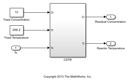
We want to transition from a residual concentration of 8.57 kmol/m^3 initially down to 2 kmol/m^3. To understand how the process dynamics evolve with the residual concentration Cr, find the equilibrium conditions for five values of Cr between 8.57 and 2 and linearize the process dynamics around each equilibrium. Log the reactor and coolant temperatures at each equilibrium point.

CrEQ = linspace(8.57,2,5)';  % concentrations
TrEQ = zeros(5,1);           % reactor temperatures
TcEQ = zeros(5,1);           % coolant temperatures

% Specify trim conditions
opspec = operspec('rct_CSTR_OL',5);
for k=1:5
   % Set desired residual concentration
   opspec(k).Outputs(1).y = CrEQ(k);
   opspec(k).Outputs(1).Known = true;
end

% Compute equilibrium condition and log corresponding temperatures
[op,report] = findop('rct_CSTR_OL',opspec,...
   findopOptions('DisplayReport','off'));
for k=1:5
   TrEQ(k) = report(k).Outputs(2).y;
   TcEQ(k) = op(k).Inputs.u;
end

% Linearize process dynamics at trim conditions
G = linearize('rct_CSTR_OL', 'rct_CSTR_OL/CSTR', op);
G.InputName = {'Cf','Tf','Tc'};
G.OutputName = {'Cr','Tr'};

Plot the reactor and coolant temperatures at equilibrium as a function of concentration.

subplot(311), plot(CrEQ,'b-*'), grid, title('Residual concentration'), ylabel('CrEQ')
subplot(312), plot(TrEQ,'b-*'), grid, title('Reactor temperature'), ylabel('TrEQ')
subplot(313), plot(TcEQ,'b-*'), grid, title('Coolant temperature'), ylabel('TcEQ')

An open-loop control strategy consists of following the coolant temperature profile above to smoothly transition between the Cr=8.57 and Cr=2 equilibria. However, this strategy is doomed by the fact that the reaction is unstable in the mid range and must be properly cooled to avoid thermal runaway. This is confirmed by inspecting the poles of the linearized models for the five equilibrium points considered above (three out of the five models are unstable).

pole(G)

ans(:,:,1) =

  -0.5225 + 0.0000i
  -0.8952 + 0.0000i


ans(:,:,2) =

   0.1733 + 0.0000i
  -0.8866 + 0.0000i


ans(:,:,3) =

   0.5114 + 0.0000i
  -0.8229 + 0.0000i


ans(:,:,4) =

   0.0453 + 0.0000i
  -0.4991 + 0.0000i


ans(:,:,5) =

  -1.1077 + 1.0901i
  -1.1077 - 1.0901i

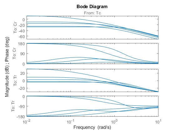
The Bode plot further highlights the significant variations in plant dynamics while transitioning from Cr=8.57 to Cr=2.

clf, bode(G(:,'Tc'),{0.01,10})

Feedback Control Strategy

To prevent thermal runaway while ramping down the residual concentration, use feedback control to adjust the coolant temperature Tc based on measurements of the residual concentration Cr and reactor temperature Tr. For this application, we use a cascade control architecture where the inner loop regulates the reactor temperature and the outer loop tracks the concentration setpoint. Both feedback loops are digital with a sampling period of 0.5 minutes.

open_system('rct_CSTR')

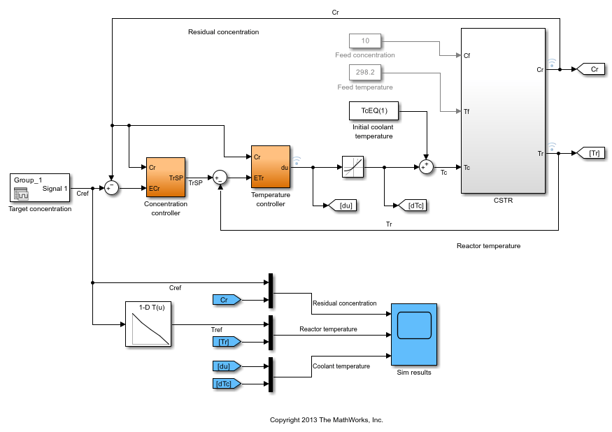
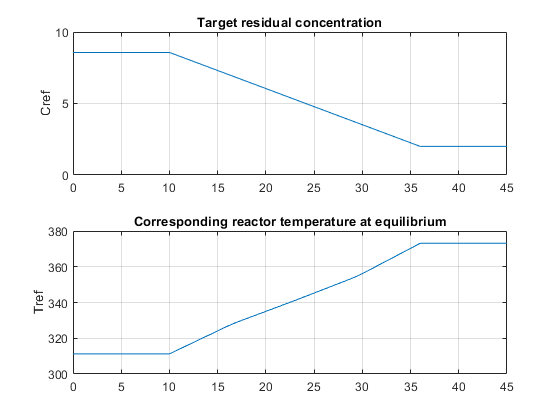
The target concentration Cref ramps down from 8.57 kmol/m^3 at t=10 to 2 kmol/m^3 at t=36 (the transition lasts 26 minutes). The corresponding profile Tref for the reactor temperature is obtained by interpolating the equilibrium values TrEQ from trim analysis. The controller computes the coolant temperature adjustment dTc relative to the initial equilibrium value TcEQ(1)=297.98 for Cr=8.57. Note that the model is set up so that initially, the output TrSP of the "Concentration controller" block matches the reactor temperature, the adjustment dTc is zero, and the coolant temperature Tc is at its equilibrium value TcEQ(1).

clf
t = [0 10:36 45];
C = interp1([0 10 36 45],[8.57 8.57 2 2],t);
subplot(211), plot(t,C), grid, set(gca,'ylim',[0 10])
title('Target residual concentration'), ylabel('Cref')
subplot(212), plot(t,interp1(CrEQ,TrEQ,C))
title('Corresponding reactor temperature at equilibrium'), ylabel('Tref'), grid

Control Objectives

Use TuningGoal objects to capture the design requirements. First, Cr should follow setpoints Cref with a response time of about 5 minutes.

R1 = TuningGoal.Tracking('Cref','Cr',5);

The inner loop (temperature) should stabilize the reaction dynamics with sufficient damping and fast enough decay.

MinDecay = 0.2;
MinDamping = 0.5;
% Constrain closed-loop poles of inner loop with the outer loop open
R2 = TuningGoal.Poles('Tc',MinDecay,MinDamping);
R2.Openings = 'TrSP';

The Rate Limit block at the controller output specifies that the coolant temperature Tc cannot vary faster than 10 degrees per minute. This is a severe limitation on the controller authority which, when ignored, can lead to poor performance or instability. To take this rate limit into account, observe that Cref varies at a rate of 0.25 kmol/m^3/min. To ensure that Tc does not vary faster than 10 degrees/min, the gain from Cref to Tc should be less than 10/0.25=40.

R3 = TuningGoal.Gain('Cref','Tc',40);

Finally, require at least 7 dB of gain margin and 45 degrees of phase margin at the plant input Tc.

R4 = TuningGoal.Margins('Tc',7,45);

Gain-Scheduled Controller

To achieve these requirements, we use a PI controller in the outer loop and a lead compensator in the inner loop. Due to the slow sampling rate, the lead compensator is needed to adequately stabilize the chemical reaction at the mid-range concentration Cr = 5.28 kmol/m^3/min. Because the reaction dynamics vary substantially with concentration, we further schedule the controller gains as a function of concentration. This is modeled in Simulink using Lookup Table blocks as shown in Figures 1 and 2.

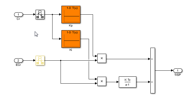
Figure 1: Gain-scheduled PI controller for concentration loop.

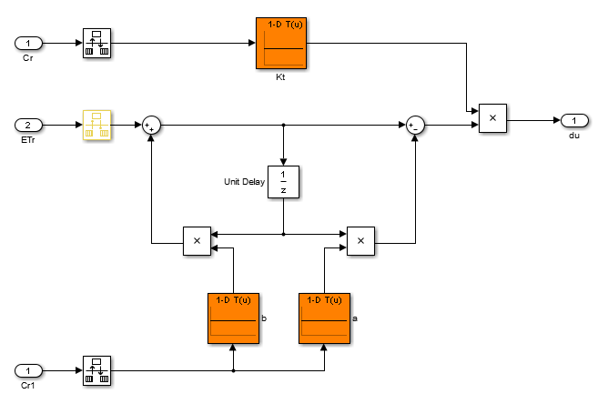
Figure 2: Gain-scheduled lead compensator for temperature loop.

Tuning this gain-scheduled controller amounts to tuning the look-up table data over a range of concentration values. Rather than tuning individual look-up table entries, parameterize the controller gains Kp,Ki,Kt,a,b as quadratic polynomials in Cr, for example,

Besides reducing the number of variables to tune, this approach ensures smooth gain transitions as Cr varies. Using systune, you can automatically tune the coefficients to meet the requirements R1-R4 at the five equilibrium points computed above. This amounts to tuning the gain-scheduled controller at five design points along the Cref trajectory. Use the tunableSurface object to parameterize each gain as a quadratic function of Cr. The "tuning grid" is set to the five concentrations CrEQ and the basis functions for the quadratic parameterization are . Most gains are initialized to be identically zero.

TuningGrid = struct('Cr',CrEQ);
ShapeFcn = @(Cr) [Cr , Cr^2];

Kp = tunableSurface('Kp', 0, TuningGrid, ShapeFcn);
Ki = tunableSurface('Ki', -2, TuningGrid, ShapeFcn);
Kt = tunableSurface('Kt', 0, TuningGrid, ShapeFcn);
a = tunableSurface('a', 0, TuningGrid, ShapeFcn);
b = tunableSurface('b', 0, TuningGrid, ShapeFcn);

Controller Tuning

Because the target bandwidth is within a decade of the Nyquist frequency, it is easier to tune the controller directly in the discrete domain. Discretize the linearized process dynamics with sample time of 0.5 minutes. Use the ZOH method to reflect how the digital controller interacts with the continuous-time plant.

Ts = 0.5;
Gd = c2d(G,Ts);

Create an slTuner interface for tuning the quadratic gain schedules introduced above. Use block substitution to replace the nonlinear plant model by the five discretized linear models Gd obtained at the design points CrEQ. Use setBlockParam to associate the tunable gain functions Kp, Ki, Kt, a, b with the Lookup Table blocks of the same name.

BlockSubs = struct('Name','rct_CSTR/CSTR','Value',Gd);
ST0 = slTuner('rct_CSTR',{'Kp','Ki','Kt','a','b'},BlockSubs);
ST0.Ts = Ts;  % sample time for tuning

% Register points of interest
ST0.addPoint({'Cref','Cr','Tr','TrSP','Tc'})

% Parameterize look-up table blocks
ST0.setBlockParam('Kp',Kp);
ST0.setBlockParam('Ki',Ki);
ST0.setBlockParam('Kt',Kt);
ST0.setBlockParam('a',a);
ST0.setBlockParam('b',b);

You can now use systune to tune the controller coefficients against the requirements R1-R4. Make the stability margin requirement a hard constraints and optimize the remaining requirements.

ST = systune(ST0,[R1 R2 R3],R4);

Final: Soft = 1.23, Hard = 0.99888, Iterations = 214

The resulting design satisfies the hard constraint (Hard<1) and nearly satisfies the remaining requirements (Soft close to 1). To validate this design, simulate the responses to a ramp in concentration with the same slope as Cref. Each plot shows the linear responses at the five design points CrEQ.

t = 0:Ts:20;
uC = interp1([0 2 5 20],(-0.25)*[0 0 3 3],t);
subplot(211), lsim(getIOTransfer(ST,'Cref','Cr'),uC)
grid, set(gca,'ylim',[-1.5 0.5]), title('Residual concentration')
subplot(212), lsim(getIOTransfer(ST,'Cref','Tc'),uC)
grid, title('Coolant temperature variation')

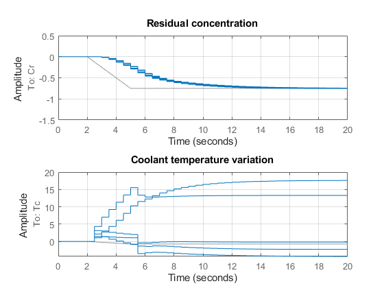
Note that rate of change of the coolant temperature remains within the physical limits (10 degrees per minute or 5 degrees per sample period).

Controller Validation

Inspect how each gain varies with Cr during the transition.

% Access tuned gain schedules
TGS = getBlockParam(ST);

% Plot gain profiles
clf
subplot(321), viewSurf(TGS.Kp), ylabel('Kp')
subplot(322), viewSurf(TGS.Ki), ylabel('Ki')
subplot(323), viewSurf(TGS.Kt), ylabel('Kt')
subplot(324), viewSurf(TGS.a), ylabel('a')
subplot(325), viewSurf(TGS.b), ylabel('b')

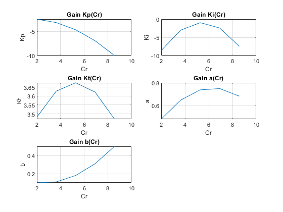
To validate the gain-scheduled controller in Simulink, first use writeBlockValue to apply the tuning results to the Simulink model. For each Lookup Table block, this evaluates the corresponding quadratic gain formula at the table breakpoints and updates the table data accordingly.

writeBlockValue(ST)

Next push the Play button to simulate the response with the tuned gain schedules. The simulation results appear in Figure 3. The gain-scheduled controller successfully drives the reaction through the transition with adequate response time and no saturation of the rate limits (controller output du matches effective temperature variation dTc). The reactor temperature stays close to its equilibrium value Tref, indicating that the controller keeps the reaction near equilibrium while preventing thermal runaway.

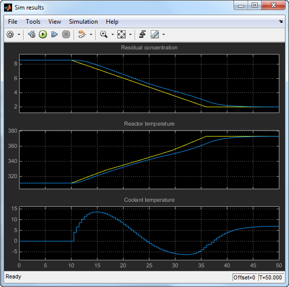
Figure 3: Transition with gain-scheduled cascade controller.

Controller Tuning in MATLAB

Alternatively, you can tune the gain schedules directly in MATLAB® without using the slTuner interface. First parameterize the gains as quadratic functions of Cr as done above.

TuningGrid = struct('Cr',CrEQ);
ShapeFcn = @(Cr) [Cr , Cr^2];

Kp = tunableSurface('Kp', 0, TuningGrid, ShapeFcn);
Ki = tunableSurface('Ki', -2, TuningGrid, ShapeFcn);
Kt = tunableSurface('Kt', 0, TuningGrid, ShapeFcn);
a = tunableSurface('a', 0, TuningGrid, ShapeFcn);
b = tunableSurface('b', 0, TuningGrid, ShapeFcn);

Use these gains to build the PI and lead controllers.

PI = pid(Kp,Ki,'Ts',Ts,'TimeUnit','min');
PI.u = 'ECr';   PI.y = 'TrSP';

LEAD = Kt * tf([1 -a],[1 -b],Ts,'TimeUnit','min');
LEAD.u = 'ETr';   LEAD.y = 'Tc';

Use connect to build a closed-loop model of the overall control system at the five design points. Mark the controller outputs TrSP and Tc as "analysis points" so that loops can be opened and stability margins evaluated at these locations. The closed-loop model T0 is a 5-by-1 array of linear models depending on the tunable coefficients of Kp,Ki,Kt,a,b. Each model is discrete and sampled every half minute.

Gd.TimeUnit = 'min';
S1 = sumblk('ECr = Cref - Cr');
S2 = sumblk('ETr = TrSP - Tr');
T0 = connect(Gd(:,'Tc'),LEAD,PI,S1,S2,'Cref','Cr',{'TrSP','Tc'});

Finally, use systune to tune the gain schedule coefficients.

T = systune(T0,[R1 R2 R3],R4);

Final: Soft = 1.23, Hard = 0.99966, Iterations = 198

The result is similar to the one obtained above. Confirm by plotting the gains as a function of Cr using the tuned coefficients in T.

clf
subplot(321), viewSurf(setBlockValue(Kp,T)), ylabel('Kp')
subplot(322), viewSurf(setBlockValue(Ki,T)), ylabel('Ki')
subplot(323), viewSurf(setBlockValue(Kt,T)), ylabel('Kt')
subplot(324), viewSurf(setBlockValue(a,T)), ylabel('a')
subplot(325), viewSurf(setBlockValue(b,T)), ylabel('b')

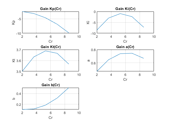
You can further validate the design by simulating the linear responses at each design point. However, you need to return to Simulink to simulate the nonlinear response of the gain-scheduled controller.