Tuning of Gain-Scheduled Three-Loop Autopilot
This example uses systune to generate smooth gain schedules for a three-loop autopilot.
Airframe Model and Three-Loop Autopilot
This example uses a three-degree-of-freedom model of the pitch axis dynamics of an airframe. The states are the Earth coordinates  , the body coordinates
  , the pitch angle
  , and the pitch rate
  . The following figure summarizes the relationship between the inertial and body frames, the flight path angle
  , the incidence angle
  , and the pitch angle
  .
.
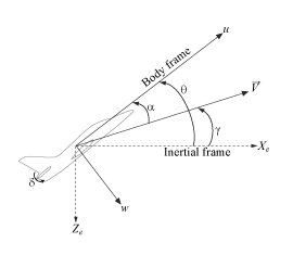
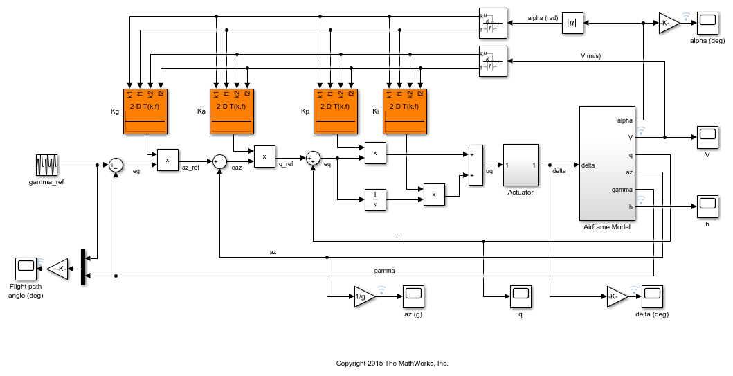
We use a classic three-loop autopilot structure to control the flight path angle  . This autopilot adjusts the flight path by delivering adequate bursts of normal acceleration
  (acceleration along
  ). In turn, normal acceleration is produced by adjusting the elevator deflection
  to cause pitching and vary the amount of lift. The autopilot uses Proportional-Integral (PI) control in the pitch rate loop
  and proportional control in the
  and
and  loops. The closed-loop system (airframe and autopilot) are modeled in Simulink®.
open_system('rct_airframeGS')
Autopilot Gain Scheduling
The airframe dynamics are nonlinear and the aerodynamic forces and moments depend on speed  and incidence
  . To obtain suitable performance throughout the
  flight envelope, the autopilot gains must be adjusted as a function of
  and
and  to compensate for changes in plant dynamics. This adjustment process is called "gain scheduling" and
  are called the scheduling variables. In the Simulink model, gain schedules are implemented as look-up tables driven by measurements of
  and
and  .
.
Gain scheduling is a linear technique for controlling nonlinear or time-varying plants. The idea is to compute linear approximations of the plant at various operating conditions, tune the controller gains at each operating condition, and swap gains as a function of operating condition during operation. Conventional gain scheduling involves the following three major steps.
Trim and linearize the plant at each operating condition
Tune the controller gains for the linearized dynamics at each operating condition
Reconcile the gain values to provide smooth transition between operating conditions.
In this example, you combine steps 2 and 3 by parameterizing the autopilot gains as first-order polynomials in  and directly tuning the polynomial coefficients for the entire flight envelope. This approach eliminates step 3 and guarantees smooth gain variations as a function of
  and
and  . Moreover, the gain schedule coefficients can be automatically tuned with
 systune.
Trimming and Linearization
Assume that the incidence  varies between -20 and 20 degrees and that the speed
  varies between 700 and 1400 m/s. When neglecting gravity, the airframe dynamics are symmetric in
  . Therefore, consider only positive values of
  . Use a 5-by-9 grid of linearly spaced
  pairs to cover the flight envelope.
nA = 5;  % number of alpha values
nV = 9;  % number of V values
[alpha,V] = ndgrid(linspace(0,20,nA)*pi/180,linspace(700,1400,nV));
For each flight condition  , linearize the airframe dynamics at trim (zero normal acceleration and pitching moment). This requires computing the elevator deflection
  and pitch rate
  that result in steady
  and
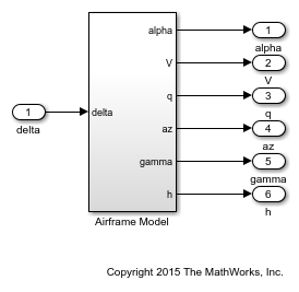
and  . To do this, first isolate the airframe model in a separate Simulink model.
mdl = 'rct_airframeTRIM';
open_system(mdl)
Use operspec to specify the trim condition, use findop to compute the trim values of  and
and  , and linearize the airframe dynamics for the resulting operating points. For details, see Trim and Linearize an Airframe (Simulink Control Design). Repeat these steps for the 45 flight conditions
  .
.
Compute the trim condition for each  pair.
pair.
for ct=1:nA*nV
   alpha_ini = alpha(ct);      % Incidence [rad]
   v_ini = V(ct);              % Speed [m/s]

   % Specify trim condition
   opspec(ct) = operspec(mdl);
   % Xe,Ze: known, not steady
   opspec(ct).States(1).Known = [1;1];
   opspec(ct).States(1).SteadyState = [0;0];
   % u,w: known, w steady
   opspec(ct).States(3).Known = [1 1];
   opspec(ct).States(3).SteadyState = [0 1];
   % theta: known, not steady
   opspec(ct).States(2).Known = 1;
   opspec(ct).States(2).SteadyState = 0;
   % q: unknown, steady
   opspec(ct).States(4).Known = 0;
   opspec(ct).States(4).SteadyState = 1;
end
opspec = reshape(opspec,[nA nV]);
Trim the model for the given specifications.
Options = findopOptions('DisplayReport','off');
op = findop(mdl,opspec,Options);
Linearize the model at the trim conditions.
G = linearize(mdl,op);
G.u = 'delta';
G.y = {'alpha','V','q','az','gamma','h'};
G.SamplingGrid = struct('alpha',alpha,'V',V);
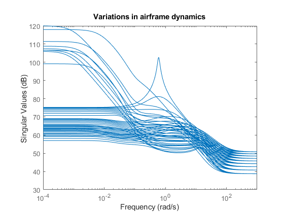
This process produces a 5-by-9 array of linearized plant models at the 45 flight conditions  . The plant dynamics vary substantially across the flight envelope.
sigma(G)
title('Variations in airframe dynamics')
Tunable Gain Surface
The autopilot consists of four gains  to be "scheduled" (adjusted) as a function of
  and
and  . Practically, this means tuning 88 values in each of the corresponding four look-up tables. Rather than tuning each table entry separately, parameterize the gains as a two-dimensional gain surfaces, for example, surfaces with a simple multi-linear dependence on
  and
and  :
:
 .
.
This cuts the number of variables from 88 down to 4 for each lookup table. Use the tunableSurface object to parameterize each gain surface. Note that:
TuningGridspecifies the "tuning grid" (design points). This grid should match the one used for linearization but needs not match the loop-up table breakpointsShapeFcnspecifies the basis functions for the surface parameterization ( ,
,  , and
, and  )
)
Each surface is initialized to a constant gain using the tuning results for  = 10 deg and
  = 1050 m/s (mid-range design).
TuningGrid = struct('alpha',alpha,'V',V);
ShapeFcn = @(alpha,V) [alpha,V,alpha*V];

Kp = tunableSurface('Kp',0.1, TuningGrid,ShapeFcn);
Ki = tunableSurface('Ki',2, TuningGrid,ShapeFcn);
Ka = tunableSurface('Ka',0.001, TuningGrid,ShapeFcn);
Kg = tunableSurface('Kg',-1000, TuningGrid,ShapeFcn);
Next create an slTuner interface for tuning the gain surfaces. Use block substitution to replace the nonlinear plant model by the linearized models over the tuning grid. Use setBlockParam to associate the tunable gain surfaces Kp, Ki, Ka, Kg with the Interpolation blocks of the same name.
BlockSubs = struct('Name','rct_airframeGS/Airframe Model','Value',G);
ST0 = slTuner('rct_airframeGS',{'Kp','Ki','Ka','Kg'},BlockSubs);

% Register points of interest
ST0.addPoint({'az_ref','az','gamma_ref','gamma','delta'})

% Parameterize look-up table blocks
ST0.setBlockParam('Kp',Kp,'Ki',Ki,'Ka',Ka,'Kg',Kg);
Autopilot Tuning
systune can automatically tune the gain surface coefficients for the entire flight envelope. Use TuningGoal objects to specify the performance objectives:
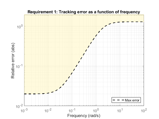
 loop: Track the setpoint with a 1 second response time, less than 2% steady-state error, and less than 30% peak error.
Req1 = TuningGoal.Tracking('gamma_ref','gamma',1,0.02,1.3);
viewGoal(Req1)
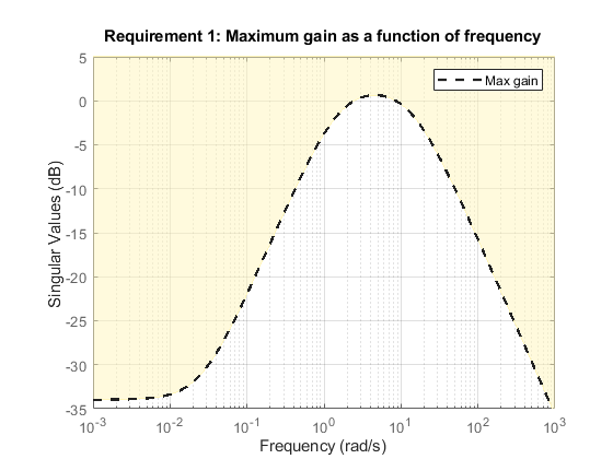
 loop: Ensure good disturbance rejection at low frequency (to track acceleration demands) and past 10 rad/s (to be insensitive to measurement noise). The disturbance is injected at the
 az_reflocation.
RejectionProfile = frd([0.02 0.02 1.2 1.2 0.1],[0 0.02 2 15 150]);
Req2 = TuningGoal.Gain('az_ref','az',RejectionProfile);
viewGoal(Req2)
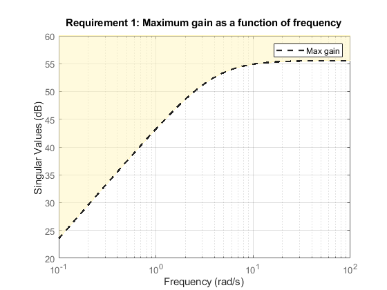
 loop: Ensure good disturbance rejection up to 10 rad/s. The disturbance is injected at the plant input
 delta.
Req3 = TuningGoal.Gain('delta','az',600*tf([0.25 0],[0.25 1]));
viewGoal(Req3)
Transients: Ensure a minimum damping ratio of 0.35 for oscillation-free transients
MinDamping = 0.35;
Req4 = TuningGoal.Poles(0,MinDamping);
Using systune, tune the 16 gain surface coefficients to best meet these performance requirements at all 45 flight conditions.
ST = systune(ST0,[Req1 Req2 Req3 Req4]);
Final: Soft = 1.13, Hard = -Inf, Iterations = 57
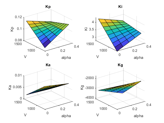
The final value of the combined objective is close to 1, indicating that all requirements are nearly met. Visualize the resulting gain surfaces.
% Get tuned gain surfaces.
TGS = getBlockParam(ST);

% Plot gain surfaces.
clf
subplot(2,2,1)
viewSurf(TGS.Kp)
title('Kp')
subplot(2,2,2)
viewSurf(TGS.Ki)
title('Ki')
subplot(2,2,3)
viewSurf(TGS.Ka)
title('Ka')
subplot(2,2,4)
viewSurf(TGS.Kg)
title('Kg')
Validation
First validate the tuned autopilot at the 45 flight conditions considered above. Plot the response to a step change in flight path angle and the response to a step disturbance in elevator deflection.
clf
subplot(2,1,1)
step(getIOTransfer(ST,'gamma_ref','gamma'),5)
grid
title('Tracking of step change in flight path angle')
subplot(2,1,2)
step(getIOTransfer(ST,'delta','az'),3)
grid
title('Rejection of step disturbance at plant input')
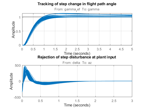
The responses are satisfactory at all flight conditions. Next validate the autopilot against the nonlinear airframe model. First use writeBlockValue to apply the tuning results to the Simulink model. This evaluates each gain surface formula at the breakpoints specified in the two Prelookup blocks and writes the result in the corresponding Interpolation block.
writeBlockValue(ST)
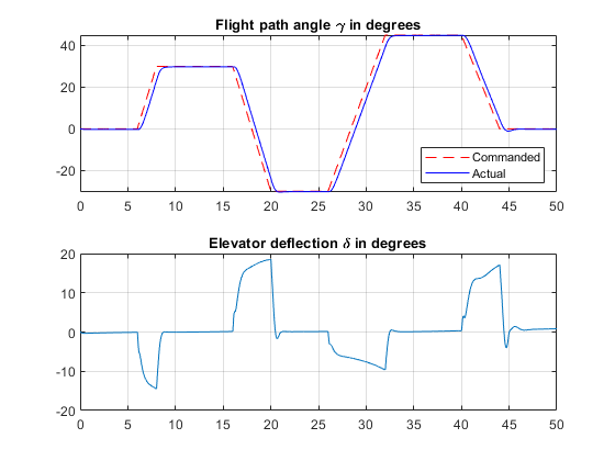
Simulate the autopilot performance for a maneuver that takes the airframe through a large portion of its flight envelope. The code below is equivalent to pressing the Play button in the Simulink model and inspecting the responses in the Scope blocks.
% Specify the initial conditions.
h_ini = 1000;
alpha_ini = 0;
v_ini = 700;

% Simulate the model.
SimOut = sim('rct_airframeGS', 'ReturnWorkspaceOutputs', 'on');

% Extract simulation data.
SimData = get(SimOut,'sigsOut');
Sim_gamma = getElement(SimData,'gamma');
Sim_alpha = getElement(SimData,'alpha');
Sim_V = getElement(SimData,'V');
Sim_delta = getElement(SimData,'delta');
Sim_h = getElement(SimData,'h');
Sim_az = getElement(SimData,'az');
t = Sim_gamma.Values.Time;

% Plot the main flight variables.
clf
subplot(2,1,1)
plot(t,Sim_gamma.Values.Data(:,1),'r--',t,Sim_gamma.Values.Data(:,2),'b')
grid
legend('Commanded','Actual','location','SouthEast')
title('Flight path angle \gamma in degrees')
subplot(2,1,2)
plot(t,Sim_delta.Values.Data)
grid
title('Elevator deflection \delta in degrees')
subplot(2,1,1)
plot(t,Sim_alpha.Values.Data)
grid
title('Incidence \alpha in degrees')
subplot(2,1,2)
plot(t,Sim_V.Values.Data)
grid
title('Speed V in m/s')

subplot(2,1,1)
plot(t,Sim_h.Values.Data)
grid
title('Altitude h in meters')
subplot(2,1,2)
plot(t,Sim_az.Values.Data)
grid
title('Normal acceleration a_z in g''s')
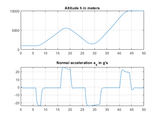
Tracking of the flight path angle profile remains good throughout the maneuver. Note that the variations in incidence  and speed
  cover most of the flight envelope considered here ([-20,20] degrees for
  and [700,1400] for
  ). And while the autopilot was tuned for a nominal altitude of 3000 m, it fares well for altitude changing from 1,000 to 10,000 m.
The nonlinear simulation results confirm that the gain-scheduled autopilot delivers consistently high performance throughout the flight envelope. The "gain surface tuning" procedure provides simple explicit formulas for the gain dependence on the scheduling variables. Instead of using look-up tables, you can use these formulas directly for an more memory-efficient hardware implementation.
See Also
slTuner (Simulink Control Design) | tunableSurface | setBlockParam (Simulink Control Design)