Gain-Scheduled LQG Controller

LPV Plant

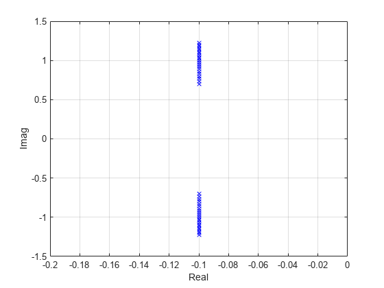
The LPV plant is a second-order model that depends on the parameter $\mathit{p}$. The system has two lightly damped poles for frozen (constant) values of $\mathit{p}$. The plant equations are

where the parameter $\mathit{p}$ satisfies $\left|\mathit{p}\right|\le 1$.

G = lpvss('p',@GFCN);

Display the poles at "frozen" parameter values.

pval = -1:0.1:1;
Gs = sample(G,0,pval);
Gpole = pole(Gs);
Gpole = Gpole(:);

plot(real(Gpole),imag(Gpole),'bx');
axis([-0.2 0 -1.5 1.5]);
xlabel('Real');
ylabel('Imag')
grid on;

Gain-Scheduled LQG Controller with Integral Action

A gain-scheduled linear-quadratic-Gaussian (LQG) controller combines state feedback with a state observer and includes integral action. The observer and state feedback gains are designed using loop-transfer recovery. The scheduled controller (including integral action) corresponds to ${\mathit{K}}_{\mathit{a}}$ in Figure 1 of [1].

Augment the plant with an integrator at the input as shown in Figure 1 of [1]. The integrator is implemented with the controller. The integral action ensures good low frequency tracking and perfect rejection of constant disturbances.

Gaug = G*tf(1,[1 0]);

Construct the LPV controller using the function KFCN. For any parameter value, this function computes LQR and Kalman gains for the corresponding plant matrices.

Ka = lpvss('p', @(t,p) KFCN(t,p,Gaug));

LTI Analysis

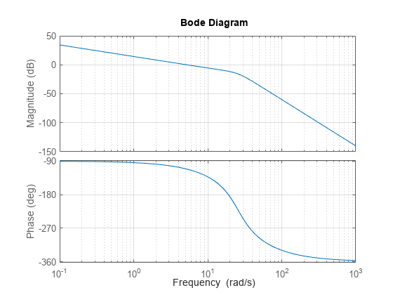
Plot the open-loop response for frozen parameter values. Note that the loops are the same at all parameter values. The scheduled controller cancels the lightly damped poles at frozen parameter values.

L = G*Ka;
Ls = sample(L,[],pval);

bode(Ls)
grid on;

The step responses for frozen parameter values show zero steady-state error, no overshoot, and a settling time of less than one second.

Ts = feedback(Ls,1);
step(Ts)
grid on;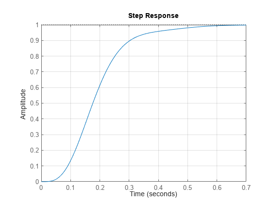

LPV Analysis

Use feedback to construct a closed-loop LPV model and plot the LPV step response for slowly-varying parameter $\mathit{p}\left(\mathit{t}\right)$. The response is similar to the LTI responses for frozen $\mathit{p}$.

T = feedback(L,1);

% Slow parameter variation
t = linspace(0,10,1000);
pt = cos(0.02*t);
step(T,t,pt)
title('Step response with p(t)=cos(0.02t)')
grid on

Next consider fast parameter variations, $\mathit{p}\left(\mathit{t}\right)=\cos \left(2\mathit{t}\right)$. The step response now shows instability.

% Fast parameter variation
t = linspace(0,100,1000);
pt = cos(2*t);
step(T,t,pt);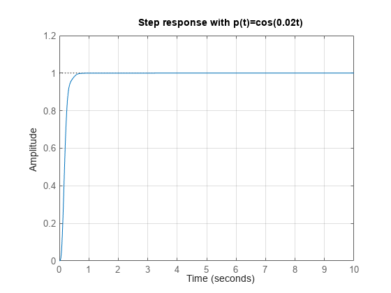
title('Step response with p(t)=cos(2t)')
grid on

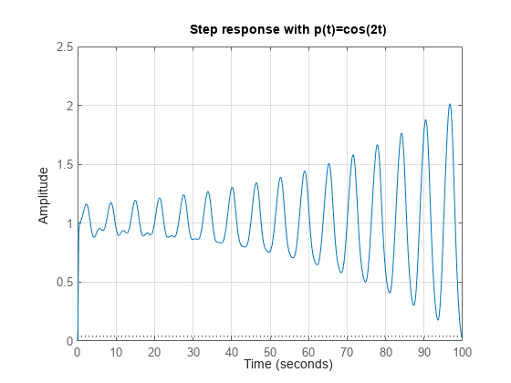
This plot corresponds to Figure 2 in [1]. The instability here results from the frozen parameters not reflecting the true dynamics. For more information, see "Potential Hazards of Gain Scheduling" in [1].

Plant and Controller Data Functions

type GFCN

function [A,B,C,D,E,dx0,x0,u0,y0,Delays] = GFCN(~,p) 

% Clip p to range [-1,1]
p = max(-1,min(p,1));

A = [0 1; -1-p/2 -0.2];
B = [0; 1];
C = [1 0];
D = 0;
E = [];
dx0 = [];
x0 = [];
u0 = [];
y0 = [];
Delays = [];

type KFCN

function [A,B,C,D,E,dx0,x0,u0,y0,Delays] = KFCN(t,p,Gaug) 
% This code solves Riccati equations and forms the gains for each value 
% of p.  This is not particularly efficient especially if used for
% simulations or real-time implementation. An alternative would be to 
% pre-solve either the Riccati equations (or the gains) on a grid of 
% parameters and then interpolate.

% Sample augmented plant to get dynamics at (t,p)
[Aaug,Baug,Caug,~] = ssdata(sample(Gaug,t,p));

% Design Parameters
N = [1; 0; 1+p/2];
mu = 0.01;
rho = 1e-8;

% Solve observer and state-feedback Riccati equations
% The observer and state-feedback gains are given by:
%   H = Sigma*(Caug)'/mu and G = (Baug)'*Z/rho;
[~,Ht] = icare(Aaug',Caug',N*N',mu);
H = Ht';
[~,G] = icare(Aaug,Baug,Caug'*Caug,rho);

% Observer / state-feedback with integral action (See Fig. 1 of [1]).
K = ss(Aaug-Baug*G-H*Caug, -H,-G,0);
Ka = tf(1,[1 0])*K;
[Ak,Bk,Ck,Dk] = ssdata(Ka);

% State-space and offset data: 
A = Ak;
B = Bk;
C = Ck;
D = Dk;
E = [];
dx0 = [];
x0 = [];
u0 = [];
y0 = [];
Delays = [];

References

[1] Shamma, J. S., and M. Athans. “Gain Scheduling: Potential Hazards and Possible Remedies.” IEEE Control Systems 12, no. 3 (June 1992): 101–7. https://doi.org/10.1109/37.165527.

[2] Shamma, "Analysis and Design of Gain Scheduled Control Systems," Ph.D. Thesis, MIT, 1988.