Hidden Couplings in Gain-Scheduled Control

LPV Plant

The following equations define the nonlinear plant.

There is a collection of equilibrium points parameterized by $\mathit{p}=\mathit{y}\in \left[-1,1\right]$.

Linearization around these equilibrium points yields the LPV model.

Use lpvss to construct this LPV plant. The data function is defined in the file lpvHCModel.m. Since ${\tanh }^{-1}\left(\mathit{p}\right)$ is infinite for $\left|\mathit{p}\right|=1$, clip $\mathit{p}$ to the range [–0.99,0.99] to stay away from singularities.

pmax = 0.99;
G = lpvss('p',@(t,p) lpvHCModel(t,p,pmax),'StateName','x');

Gain-Scheduled PI Controller

The gain-scheduled Proportional-Integral (PI) controller $\mathit{K}\left(\mathit{p}\right)$ is designed to achieve a closed loop damping ratio ${\zeta }_{\mathit{d}}=\raisebox{1ex}{$2$}\!\left/ \!\raisebox{-1ex}{$3$}\right.$ and natural frequency ${\omega }_{\mathit{d}}=1$ at each point in the domain. You can construct this controller in two different forms.

These forms are equivalent when $\mathit{p}$ is constant. However, the two forms have different input/output responses when the parameter varies in time. This example compares these two options in terms of closed-loop performance.

This example provides the code for these two controllers in the files hcKinFCN.m and hcKoutFCN.m. Use lpvss to construct the two controllers.

Kin = lpvss('p',@(t,p) hcKinFCN(t,p,pmax));
Kout = lpvss('p',@(t,p) hcKoutFCN(t,p,pmax));

Use feedback to construct LPV models of the closed-loop systems for each controller.

CLin = feedback(G*Kin,1);
CLout = feedback(G*Kout,1);

LTI Analysis

Evaluate this closed-loop response for several fixed values of $\mathit{p}$.

Sample the LPV system for five values of $\mathit{p}$.

Nvals = 5;
pvals = linspace(-0.9,0.9,Nvals);
CLinvals = sample(CLin,[],pvals);
CLoutvals = sample(CLout,[],pvals);

Plot the Bode response for fixed values of $\mathit{p}$.

bode(CLinvals,'b',CLoutvals,'r--',{1e-2,1e1});

The location of the integral gain does not affect the controller when $\mathit{p}$ is constant. Hence, the two feedback loops have identical responses.

LPV Simulation

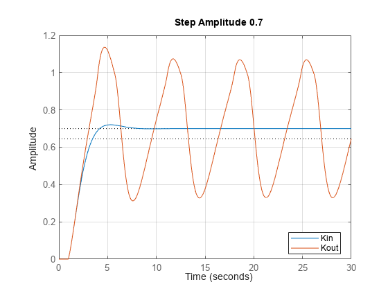
Compute the step response of the closed-loop LPV models for the two step amplitudes rstep = 0.3 and rstep = 0.7. This approximates the tracking performance of each gain-scheduled controller against the nonlinear plant. Both controllers use $\mathit{p}=\mathit{y}$ as the scheduling variable.

The feedback loop is locally unstable for $p>0.725$ with Kout while it remains locally stable for all for $p<1$ with Kin [1]. Try reproducing these results with an LPV simulation.

Tf = 30;
tsim = linspace(0,Tf,1000);
xinit = [0;0];
rstep  = 0.3;
Config = RespConfig('Amplitude',rstep,'Delay',1,'InitialState',xinit);
pFcn = @(t,x,u) tanh(x(1));
step(CLin,CLout,tsim,pFcn,Config), grid
title('Step Amplitude 0.3')
legend('Kin','Kout','location','Best')

rstep  = 0.7;
Config = RespConfig('Amplitude',rstep,'Delay',1,'InitialState',xinit);
step(CLin,CLout,tsim,pFcn,Config), grid
title('Step Amplitude 0.7')
legend('Kin','Kout','location','Best')

The LPV simulation confirms that the feedback loop remains stable with Kin (integral gain at the integrator input) but exhibits a limit cycle with Kout for large setpoint changes. This cycle is only an approximation of the true nonlinear behavior since the output $\mathit{y}$ should never exceed 1. The LPV plant model is locally linear and cannot capture the saturating behavior of the function $\tanh$.

To further assess the fidelity of the LPV model, compare with a nonlinear simulation using the true nonlinear plant.

Open the Simulink® model of the closed-loop system.

mdl = 'HiddenCouplings';
open_system(mdl)

Simulate the response with Ki at integrator output.

usey = 1; 
useKout = 1;
simout = sim('HiddenCouplings',Tf);

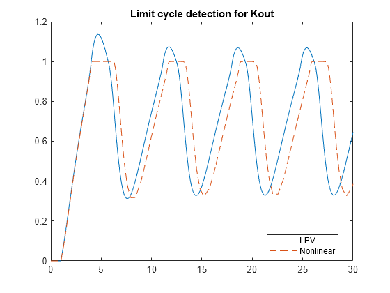
Compare the LPV and nonlinear responses with the controller Kout.

y = step(CLout,tsim,pFcn,Config);
plot(tsim,y,simout.tout,simout.y,'--')
title('Limit cycle detection for Kout')
legend('LPV','Nonlinear','location','Best')

As expected, results don't match exactly due to the strong nonlinearity of $\tanh$. Still, the LPV simulation correctly predicts the limit cycle with approximately the right period.

Scheduling on Reference Signal

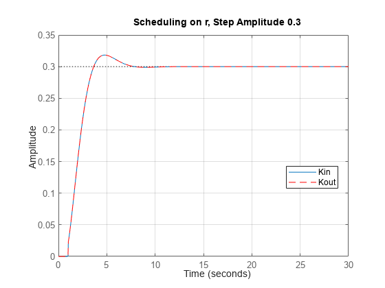
Scheduling on $\mathit{y}=\tanh \left(\mathit{x}\right)$ creates an additional feedback loop between the plant and controller via the scheduling function. In other words, the closed-loop model simulated by step is quasi-LPV and the state-dependent scheduling causes instability. Since the output $\mathit{y}$ is meant to track the reference signal $\mathit{r}$, an alternative strategy is to schedule the controller on $\mathit{r}$, which is a truly exogenous signal. You can easily compare the two strategies by replacing the parameter trajectory $\mathit{p}=\tanh \left(\mathit{x}\right)$ with $\mathit{p}=\mathit{r}$ in the step command.

rstep  = 0.3;
Config = RespConfig('Amplitude',rstep,'Delay',1,'InitialState',xinit);
r = rstep*(tsim>=1);
step(CLin,CLout,'r--',tsim,r,Config), grid
title('Scheduling on r, Step Amplitude 0.3')
legend('Kin','Kout','location','Best')

Simulate with a larger step amplitude.

rstep  = 0.7;
Config = RespConfig('Amplitude',rstep,'Delay',1,'InitialState',xinit);
step(CLin,CLout,'r--',tsim,r,Config), grid
title('Scheduling on r, Step Amplitude 0.7')
legend('Kin','Kout','location','Best')

Both controllers now remain stable and have identical performance. This is because $\mathit{p}$ is piecewise constant, which is close enough to the LTI case when both controllers are interchangeable. Save the results with Kout for comparison with the hybrid scheme discussed next.

y = step(CLout,tsim,r,Config);

Hybrid Approach

You can also use a hybrid approach where the LPV plant depends on $\mathit{p}=\mathit{y}$ and the PI controller is scheduled in $\mathit{r}$. To try this strategy, construct the LPV controller with a different parameter called pc:

Kout = lpvss('pc',@(t,p) hcKoutFCN(t,p,pmax));
CLout = feedback(G*Kout,1);

The closed-loop model now depends on two parameters p and pc. Set p to $\mathit{y}$ and pc to $\mathit{r}$ and simulate the response.

pFcn = @(t,x,u) [tanh(x(1)) ; interp1(tsim,r,t)];
yh = step(CLout,tsim,pFcn,Config);

Finally, run a nonlinear simulation with the true plant and a PI controller scheduled on $\mathit{r}$ with ${\mathit{K}}_{\mathit{i}}$ at the integrator output.

usey = 0; useKout = 1;
simout = sim('HiddenCouplings',Tf);

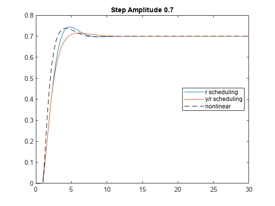
Compare the $\mathit{r}$-scheduling and hybrid scheduling schemes with the true nonlinear response.

plot(tsim,y,tsim,yh,simout.tout,simout.y,'k--')
title('Step Amplitude 0.7')
legend('r scheduling','y/r scheduling','nonlinear','location','Best')

Here scheduling both the plant and controller on $\mathit{r}$ yields a better approximation of the nonlinear response.

Plant and Controller Data Functions

type lpvHCModel

function [A,B,C,D,E,dx0,x0,u0,y0,Delays] = lpvHCModel(~,p,pmax) 
% Plant model

p = max(-pmax,min(p,pmax));
tau = atanh(p);

A = -1;
B = 1;
C = 1-p^2;
D = 0;
E = [];
dx0 = [];
x0 = tau;
u0 = tau;
y0 = p;
Delays = [];

type hcKinFCN

function [A,B,C,D,E,dx0,x0,u0,y0,Delays] = hcKinFCN(~,p,pmax) 

% PI Gains
if abs(p)< pmax
    Kp = 1/3/(1-p^2);
    Ki = 1/(1-p^2);
else
    % Protect against |p|>=1
    Kp = 1/3/(1-pmax^2);
    Ki = 1/(1-pmax^2);
end

% State-space and offset data: Ki at the input
A = 0;
B = Ki;
C = 1;
D = Kp;
E = [];
dx0 = [];
x0 = [];
u0 = [];
y0 = [];
Delays = [];

type hcKoutFCN

function [A,B,C,D,E,dx0,x0,u0,y0,Delays] = hcKoutFCN(~,p,pmax) 

% PI Gains
if abs(p)< pmax
    Kp = 1/3/(1-p^2);
    Ki = 1/(1-p^2);
else
    % Protect against |p|>=1
    Kp = 1/3/(1-pmax^2);
    Ki = 1/(1-pmax^2);
end

% State-space and offset data: Ki at the output
A = 0;
B = 1;
C = Ki;
D = Kp;
E = [];
dx0 = [];
x0 = [];
u0 = [];
y0 = [];
Delays = [];

References

Rugh, Wilson J., and Jeff S. Shamma. “Research on Gain Scheduling.” Automatica 36, no. 10 (October 2000): 1401–25. https://doi.org/10.1016/S0005-1098(00)00058-3.