MIMO Control of Diesel Engine
This example uses systune to design and tune a MIMO controller for a Diesel engine. The controller is tuned in discrete time for a single operating condition.
Diesel Engine Model
Modern Diesel engines use a variable geometry turbocharger (VGT) and exhaust gas recirculation (EGR) to reduce emissions. Tight control of the VGT boost pressure and EGR massflow is necessary to meet strict emission targets. This example shows how to design and tune a MIMO controller that regulates these two variables when the engine operates at 2100 rpm with a fuel mass of 12 mg per injection-cylinder.
open_system('rct_diesel')
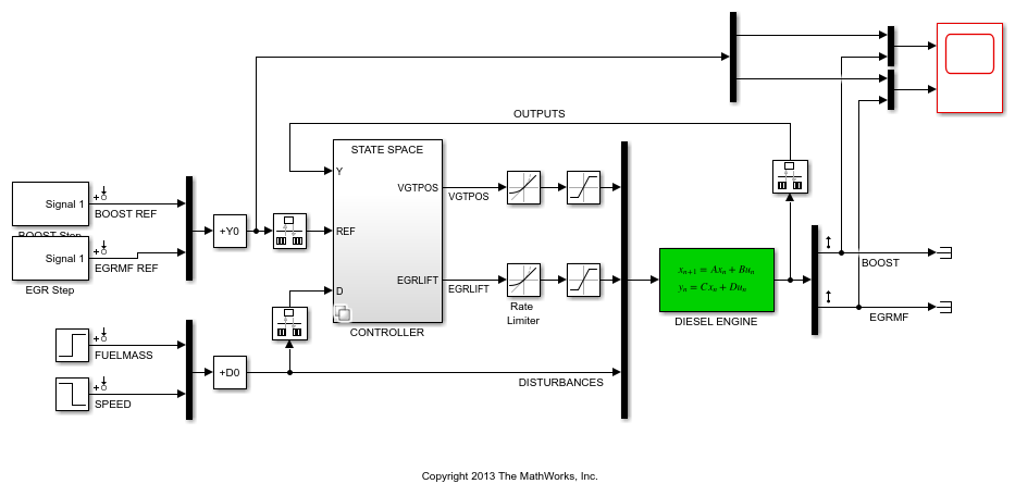
The VGT/EGR control system is modeled in Simulink®. The controller adjusts the positions EGRLIFT and VGTPOS of the EGR and VGT valves. It has access to the boost pressure and EGR massflow targets and measured values, as well as fuel mass and engine speed measurements. Both valves have rate and saturation limits. The plant model is sampled every 0.1 seconds and the control signals EGRLIFT and VGTPOS are refreshed every 0.2 seconds. This example considers step changes of +10 KPa in boost pressure and +3 g/s in EGR massflow, and disturbances of +5 mg in fuel mass and -200 rpm in speed.
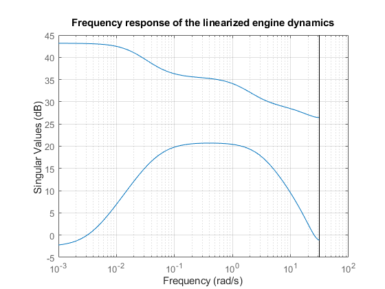
For the operating condition under consideration, we used System Identification to derive a linear model of the engine from experimental data. The frequency response from the manipulated variables EGRLIFT and VGTPOS to the controlled variables BOOST and EGR MF appears below. Note that the plant is ill conditioned at low frequency which makes independent control of boost pressure and EGR massflow difficult.
sigma(Plant(:,1:2)), grid
title('Frequency response of the linearized engine dynamics')
Control Objectives
There are two main control objectives:
Respond to step changes in boost pressure and EGR massflow in about 5 seconds with minimum cross-coupling.
Be insensitive to (small) variations in speed and fuel mass.
Use a tracking requirement for the first objective. Specify the amplitudes of the step changes to ensure that cross-couplings are small relative to these changes.
% 5-second response time, steady-state error less than 5%
TR = TuningGoal.Tracking({'BOOST REF';'EGRMF REF'},{'BOOST';'EGRMF'},5,0.05);
TR.Name = 'Setpoint tracking';
TR.InputScaling = [10 3];
For the second objective, treat the speed and fuel mass variations as step disturbances and specify the peak amplitude and settling time of the resulting variations in boost pressure and EGR massflow. Also specify the signal amplitudes to properly reflect the relative contribution of each disturbance.
% Peak<0.5, settling time<5
DR = TuningGoal.StepRejection({'FUELMASS';'SPEED'},{'BOOST';'EGRMF'},0.5,5);
DR.Name = 'Disturbance rejection';
DR.InputScaling = [5 200];
DR.OutputScaling = [10 3];
To provide adequate robustness to unmodeled dynamics and aliasing, limit the control bandwidth and impose sufficient stability margins at both the plant inputs and outputs. Because we are dealing with 2-by-2 MIMO feedback loops, this requirement guarantees stability for gain or phase variations in each feedback channel. The gain or phase can change in both channels simultaneously, and by a different amount in each channel. See Stability Margins in Control System Tuning and TuningGoal.Margins for details.
% Roll off of -20 dB/dec past 1 rad/s
RO = TuningGoal.MaxLoopGain({'EGRLIFT','VGTPOS'},1,1);
RO.LoopScaling = 'off';
RO.Name = 'Roll-off';

% 7 dB of gain margin and 45 degrees of phase margin
M1 = TuningGoal.Margins({'EGRLIFT','VGTPOS'},7,45);
M1.Name = 'Plant input';
M2 = TuningGoal.Margins('DIESEL ENGINE',7,45);
M2.Name = 'Plant output';
Tuning of Blackbox MIMO Controller
Without a-priori knowledge of a suitable control structure, first try "blackbox" state-space controllers of various orders. The plant model has four states, so try a controller of order four or less. Here we tune a second-order controller since the "SS2" block in the Simulink model has two states.
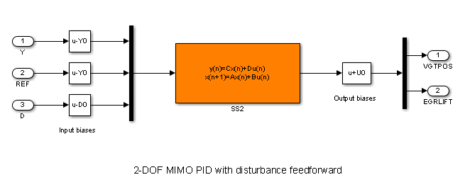
Figure 1: Second-order blackbox controller.
Use the slTuner interface to configure the Simulink model for tuning. Mark the block "SS2" as tunable, register the locations where to assess margins and loop shapes, and specify that linearization and tuning should be performed at the controller sampling rate.
ST0 = slTuner('rct_diesel','SS2');
ST0.Ts = 0.2;
addPoint(ST0,{'EGRLIFT','VGTPOS','DIESEL ENGINE'})
Now use systune to tune the state-space controller subject to our control objectives. Treat the stability margins and roll-off target as hard constraints and try to best meet the remaining objectives (soft goals). Randomize the starting point to reduce exposure to undesirable local minima.
Opt = systuneOptions('RandomStart',2);
rng(0), ST1 = systune(ST0,[TR DR],[M1 M2 RO],Opt);
Final: Soft = 1.05, Hard = 0.85503, Iterations = 347
Final: Soft = 1.05, Hard = 0.98601, Iterations = 422
Final: Soft = 1.05, Hard = 0.96663, Iterations = 404
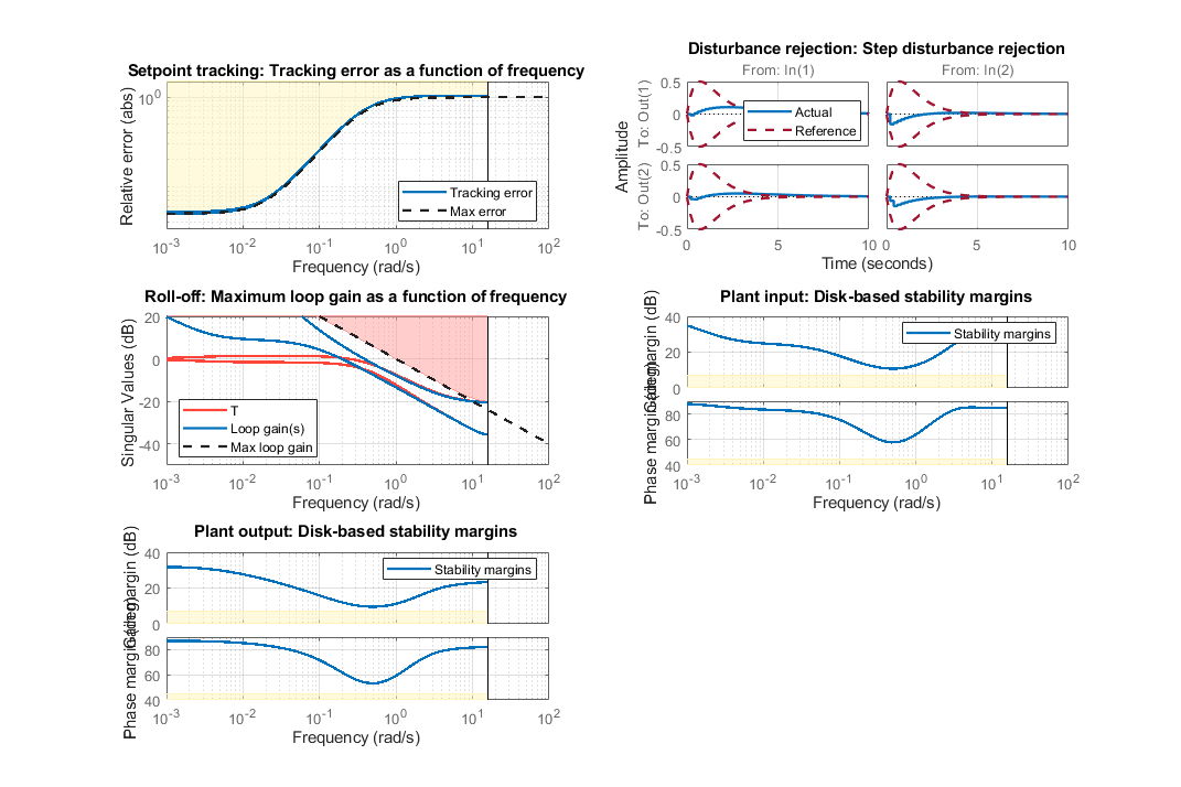
All requirements are nearly met (a requirement is satisfied when its normalized value is less than 1). Verify this graphically.
figure('Position',[10,10,1071,714])
viewGoal([TR DR RO M1 M2],ST1)
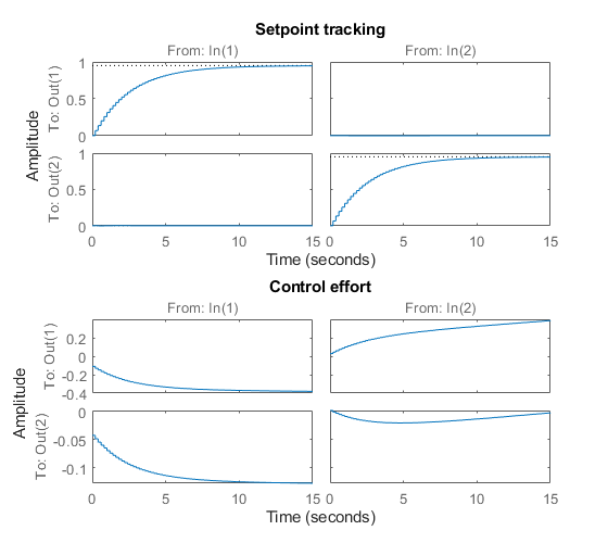
Plot the setpoint tracking and disturbance rejection responses. Scale by the signal amplitudes to show normalized effects (boost pressure changes by +10 KPa, EGR massflow by +3 g/s, fuel mass by +5 mg, and speed by -200 rpm).
figure('Position',[100,100,560,500])
T1 = getIOTransfer(ST1,{'BOOST REF';'EGRMF REF'},{'BOOST','EGRMF','EGRLIFT','VGTPOS'});
T1 = diag([1/10 1/3 1 1]) * T1 * diag([10 3]);
subplot(211), step(T1(1:2,:),15), title('Setpoint tracking')
subplot(212), step(T1(3:4,:),15), title('Control effort')
D1 = getIOTransfer(ST1,{'FUELMASS';'SPEED'},{'BOOST','EGRMF','EGRLIFT','VGTPOS'});
D1 = diag([1/10 1/3 1 1]) * D1 * diag([5 -200]);
subplot(211), step(D1(1:2,:),15), title('Disturbance rejection')
subplot(212), step(D1(3:4,:),15), title('Control effort')
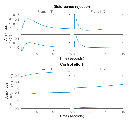
The controller responds in less than 5 seconds with minimum cross-coupling between the BOOST and EGRMF variables.
Tuning of Simplified Control Structure
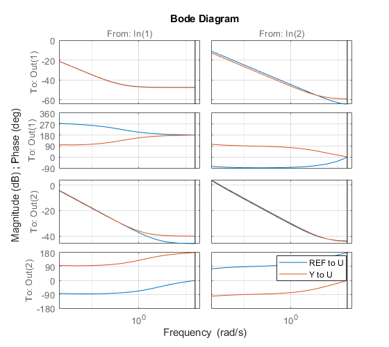
The state-space controller could be implemented as is, but it is often desirable to boil it down to a simpler, more familiar structure. To do this, get the tuned controller and inspect its frequency response.
C = getBlockValue(ST1,'SS2');

clf
bode(C(:,1:2),C(:,3:4),{.02 20}), grid
legend('REF to U','Y to U')
bodemag(C(:,5:6)), grid
title('Bode response from FUELMASS/SPEED to EGRLIFT/VGTPOS')
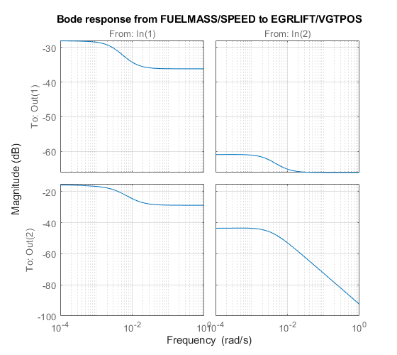
The first plot suggests that the controller essentially behaves like a PI controller acting on REF-Y (the difference between the target and actual values of the controlled variables). The second plot suggests that the transfer from measured disturbance to manipulated variables could be replaced by a gain in series with a lag network. Altogether this suggests the following simplified control structure consisting of a MIMO PI controller with a first-order disturbance feedforward.
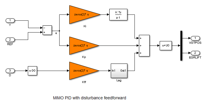
Figure 2: Simplified control structure.
Using variant subsystems, you can implement both control structures in the same Simulink model and use a variable to switch between them. Here setting MODE=2 selects the MIMO PI structure. As before, use systune to tune the three 2-by-2 gain matrices Kp, Ki, Kff in the simplified control structure.
% Select "MIMO PI" variant in "CONTROLLER" block
MODE = 2;

% Configure tuning interface
ST0 = slTuner('rct_diesel',{'Kp','Ki','Kff'});
ST0.Ts = 0.2;
addPoint(ST0,{'EGRLIFT','VGTPOS','DIESEL ENGINE'})

% Tune MIMO PI controller.
ST2 = systune(ST0,[TR DR],[M1 M2 RO]);
Final: Soft = 1.09, Hard = 0.99376, Iterations = 239
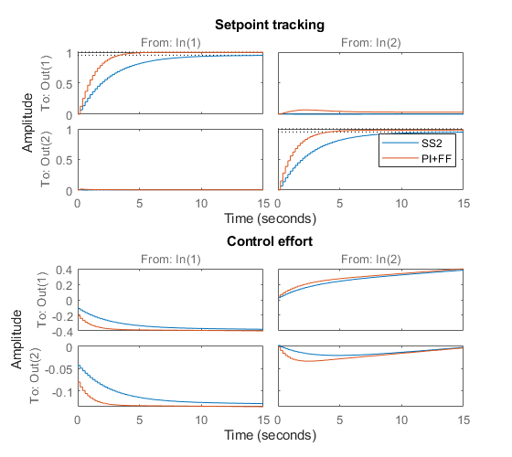
Again all requirements are nearly met. Plot the closed-loop responses and compare with the state-space design.
clf
T2 = getIOTransfer(ST2,{'BOOST REF';'EGRMF REF'},{'BOOST','EGRMF','EGRLIFT','VGTPOS'});
T2 = diag([1/10 1/3 1 1]) * T2 * diag([10 3]);
subplot(211), step(T1(1:2,:),T2(1:2,:),15), title('Setpoint tracking')
legend('SS2','PI+FF')
subplot(212), step(T1(3:4,:),T2(3:4,:),15), title('Control effort')
D2 = getIOTransfer(ST2,{'FUELMASS';'SPEED'},{'BOOST','EGRMF','EGRLIFT','VGTPOS'});
D2 = diag([1/10 1/3 1 1]) * D2 * diag([5 -200]);
subplot(211), step(D1(1:2,:),D2(1:2,:),15), title('Disturbance rejection')
legend('SS2','PI+FF')
subplot(212), step(D1(3:4,:),D2(3:4,:),15), title('Control effort')
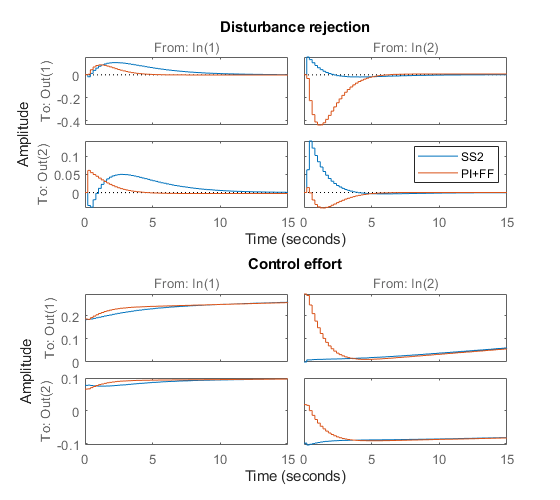
The blackbox and simplified control structures deliver similar performance. Inspect the tuned values of the PI and feedforward gains.
showTunable(ST2)
Block 1: rct_diesel/CONTROLLER/MIMO PID/Kp =

  D =
               u1          u2
   y1   -0.007966  -0.0008793
   y2    -0.02033     0.01417

Name: Kp
Static gain.

-----------------------------------

Block 2: rct_diesel/CONTROLLER/MIMO PID/Ki =

  D =
             u1        u2
   y1  -0.01056  -0.01363
   y2  -0.03002   0.04622

Name: Ki
Static gain.

-----------------------------------

Block 3: rct_diesel/CONTROLLER/MIMO PID/Kff =

  D =
               u1          u2
   y1     0.01401  -9.676e-05
   y2     0.03242   -0.001452

Name: Kff
Static gain.
Nonlinear Validation
To validate the MIMO PI controller in the Simulink model, push the tuned controller parameters to Simulink and run the simulation.
writeBlockValue(ST2)
The simulation results are shown below and confirm that the controller adequately tracks setpoint changes in boost pressure and EGR massflow and quickly rejects changes in fuel mass (at t=90) and in speed (at t=110).
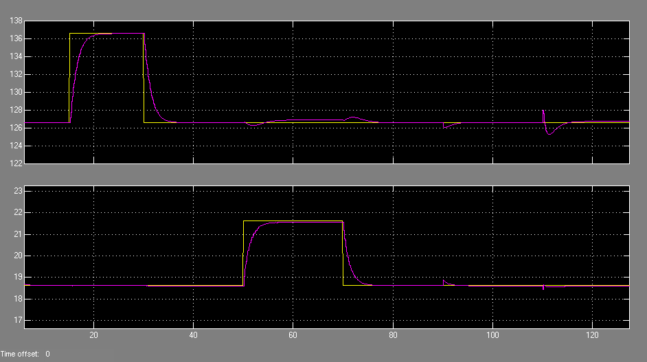
Figure 3: Simulation results with simplified controller.
See Also
systune (slTuner) (Simulink Control Design) | slTuner (Simulink Control Design) | TuningGoal.Tracking | TuningGoal.StepRejection | TuningGoal.MaxLoopGain | TuningGoal.Margins