State Estimation Using Time-Varying Kalman Filter

This example uses:

This example shows how to estimate states of linear systems using time-varying Kalman filters in Simulink®. You use the Kalman Filter block from the Control System Toolbox™ library to estimate the position and velocity of a ground vehicle based on noisy position measurements such as GPS sensor measurements. The plant model in Kalman filter has time-varying noise characteristics.

Introduction

You want to estimate the position and velocity of a ground vehicle in the north and east directions. The vehicle can move freely in the two-dimensional space without any constraints. You design a multi-purpose navigation and tracking system that can be used for any object and not just a vehicle.

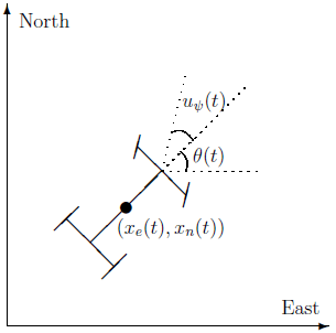
$x_e(t)$ and $x_n(t)$ are the vehicle's east and north positions from the origin, $\theta(t)$ is the vehicle orientation from east and $u_\psi(t)$ is the steering angle of the vehicle. $t$ is the continuous-time variable.

The Simulink model consists of two main parts: Vehicle model and the Kalman filter. These are explained further in the following sections.

open_system('ctrlKalmanNavigationExample');

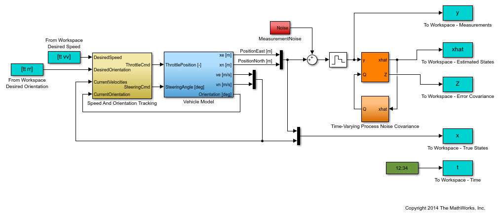
Vehicle Model

The tracked vehicle is represented with a simple point-mass model:

$\frac{d}{dt} \left[
\begin{array} {c}
 x_e(t) \\
 x_n(t) \\
 s(t) \\
 \theta(t)
\end{array} \right] = \left[
\begin{array} {c}
 s(t)\cos(\theta(t)) \\
 s(t)\sin(\theta(t)) \\
 (P \; \frac{u_T(t)}{s(t)} - A \; C_d \; s(t)^2) / m \\
 s(t) \tan(u_\psi(t)) / L
\end{array} \right]
$

where the vehicle states are:

$\begin{array} {ll}
x_e(t) \; & \textnormal{East position} \; [m] \\
x_n(t) \; & \textnormal{North position} \; [m] \\
s(t) \; & \textnormal{Speed} \; [m/s] \\
\theta(t) \; & \textnormal{Orientation from east} \; [deg] \\
\end{array}$

the vehicle parameters are:

$\begin{array} {ll}
P=100000 \; & \textnormal{Peak engine power} \; [W] \\
A=1 \; & \textnormal{Frontal area} \; [m^2] \\
C_d=0.3 \; & \textnormal{Drag coefficient} \; [Unitless] \\
m=1250 \; & \textnormal{Vehicle mass} \; [kg] \\
L=2.5 \; & \textnormal{Wheelbase length} \; [m] \\
\end{array}$

and the control inputs are:

$\begin{array} {ll}
u_T(t) \; & \textnormal{Throttle position in the range of -1 and 1} \; [Unitless] \\
u_\psi(t) \; & \textnormal{Steering angle} \; [deg] \\
\end{array}$

The longitudinal dynamics of the model ignore tire rolling resistance. The lateral dynamics of the model assume that the desired steering angle can be achieved instantaneously and ignore the yaw moment of inertia.

The car model is implemented in the ctrlKalmanNavigationExample/Vehicle Model subsystem. The Simulink model contains two PI controllers for tracking the desired orientation and speed for the car in the ctrlKalmanNavigationExample/Speed And Orientation Tracking subsystem. This allows you to specify various operating conditions for the car and test the Kalman filter performance.

Kalman Filter Design

Kalman filter is an algorithm to estimate unknown variables of interest based on a linear model. This linear model describes the evolution of the estimated variables over time in response to model initial conditions as well as known and unknown model inputs. In this example, you estimate the following parameters/variables:

$\hat{x}[n] = \left[
 \begin{array}{c}
 \hat{x}_e[n] \\
 \hat{x}_n[n] \\
 \hat{\dot{x}}_e[n] \\
 \hat{\dot{x}}_n[n]
 \end{array}
 \right]
$

where

$\begin{array} {ll}
\hat{x}_e[n] \; & \textnormal{East position estimate} \; [m] \\
\hat{x}_n[n] \; & \textnormal{North position estimate} \; [m] \\
\hat{\dot{x}}_e[n] \; & \textnormal{East velocity estimate} \; [m/s] \\
\hat{\dot{x}}_n[n] \; & \textnormal{North velocity estimate} \; [m/s] \\
\end{array}$

The $\dot{x}$ terms denote velocities and not the derivative operator. $n$ is the discrete-time index. The model used in the Kalman filter is of the form:

$\begin{array} {rl}
\hat{x}[n+1] &= A\hat{x}[n] + Gw[n] \\
y[n] &= C\hat{x}[n] + v[n]
\end{array}$

where $\hat{x}$ is the state vector, $y$ is the measurements, $w$ is the process noise, and $v$ is the measurement noise. Kalman filter assumes that $w$ and $v$ are zero-mean, independent random variables with known variances $E[ww^T]=Q$ , $E[vv^T]=R$ , and $E[wv^T]=N$ . Here, the A, G, and C matrices are:

$A = \left[
 \begin{array}{c c c c}
 1 & 0 & T_s & 0 \\
 0 & 1 & 0 & T_s \\
 0 & 0 & 1 & 0 \\
 0 & 0 & 0 & 1
 \end{array}
 \right]
$

$G = \left[
 \begin{array}{c c}
 T_s/2 & 0 \\
 0 & T_s/2 \\
 1 & 0 \\
 0 & 1
 \end{array}
 \right]
$

$C = \left[
 \begin{array}{c c c c}
 1 & 0 & 0 & 0 \\
 0 & 1 & 0 & 0
 \end{array}
 \right]
$

where $T_s=1\;[s]$

The third row of A and G model the east velocity as a random walk: $\hat{\dot{x}}_e[n+1]=\hat{\dot{x}}_e[n]+w_1[n]$ . In reality, position is a continuous-time variable and is the integral of velocity over time $\frac{d}{dt}\hat{x}_e=\hat{\dot{x}}_e$ . The first row of the A and G represent a discrete approximation to this kinematic relationship: $(\hat{x}_e[n+1]-\hat{x}_e[n])/Ts=(\hat{\dot{x}}_e[n+1]+\hat{\dot{x}}_e[n])/2$ . The second and fourth rows of the A and G represent the same relationship between the north velocity and position.

The C matrix represents that only position measurements are available. A position sensor, such as GPS, provides these measurements at the sample rate of 1Hz. The variance of the measurement noise $v$ , the R matrix, is specified as $R=50$ . Since R is specified as a scalar, the Kalman filter block assumes that the matrix R is diagonal, its diagonals are 50 and is of compatible dimensions with y. If the measurement noise is Gaussian, R=50 corresponds to 68% of the position measurements being within $\pm\sqrt{50}\;m$ or the actual position in the east and north directions. However, this assumption is not necessary for the Kalman filter.

The elements of $w$ capture how much the vehicle velocity can change over one sample time Ts. The variance of the process noise w, the Q matrix, is chosen to be time-varying. It captures the intuition that typical values of $w[n]$ are smaller when velocity is large. For instance, going from 0 to 10m/s is easier than going from 10 to 20m/s. Concretely, you use the estimated north and east velocities and a saturation function to construct Q[n]:

$f_{sat}(z)=min(max(z,25),625)$

$Q[n] = \left[
 \begin{array}{ c c }
 \displaystyle 1+\frac{250}{f_{sat}(\hat{\dot{x}}_e^2)} & 0 \\
 0 & \displaystyle 1+\frac{250}{f_{sat}(\hat{\dot{x}}_n^2)}
 \end{array}
 \right]
$

The diagonals of Q model the variance of w inversely proportional to the square of the estimated velocities. The saturation function prevents Q from becoming too large or small. The coefficient 250 is obtained from a least squares fit to 0-5, 5-10, 10-15, 15-20, 20-25m/s acceleration time data for a generic vehicle. Note that the diagonal Q choice represents a naive assumption that the velocity changes in the north and east direction are uncorrelated.

Kalman Filter Block Inputs and Setup

The 'Kalman Filter' block is in the Control System Toolbox library in Simulink. It is also in System Identification Toolbox/Estimators library. Configure the block parameters for discrete-time state estimation. Specify the following Filter Settings parameters:

Time domain: Discrete-time. Choose this option to estimate discrete-time states.

Select the Use current measurement y[n] to improve xhat[n] check box. This implements the "current estimator" variant of the discrete-time Kalman filter. This option improves the estimation accuracy and is more useful for slow sample times. However, it increases the computational cost. In addition, this Kalman filter variant has direct feedthrough, which leads to an algebraic loop if the Kalman filter is used in a feedback loop that does not contain any delays (the feedback loop itself also has direct feedthrough). The algebraic loop can further impact the simulation speed.

Click the Options tab to set the block inport and outport options:

Unselect the Add input port u check box. There are no known inputs in the plant model.

Select the Output state estimation error covariance Z check box. The Z matrix provides information about the filter's confidence in the state estimates.

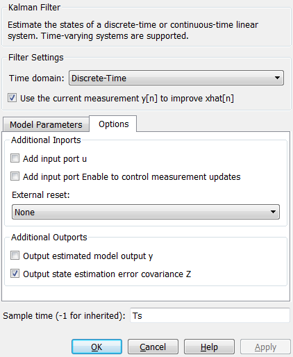
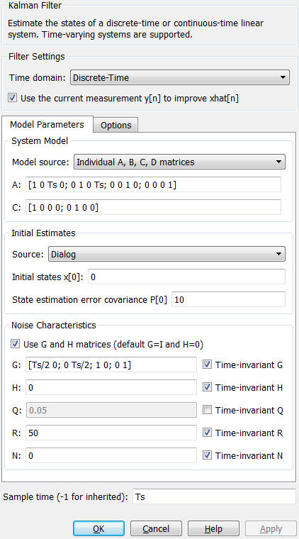
Click Model Parameters to specify the plant model and noise characteristics:

Model source: Individual A, B, C, D matrices.

A: A. The A matrix is defined earlier in this example.

C: C. The C matrix is defined earlier in this example.

Initial Estimate Source: Dialog

Initial states x[0]: 0. This represents an initial guess of 0 for the position and velocity estimates at t=0s.

State estimation error covariance P[0]: 10. Assume that the error between your initial guess x[0] and its actual value is a random variable with a standard deviation $\sqrt{10}$ .

Select the Use G and H matrices (default G=I and H=0) check box to specify a non-default G matrix.

G: G. The G matrix is defined earlier in this example.

H: 0. The process noise does not impact the measurements y entering the Kalman filter block.

Unselect the Time-invariant Q check box. The Q matrix is time-varying and is supplied through the block inport Q. The block uses a time-varying Kalman filter due to this setting. You can select this option to use a time-invariant Kalman filter. A time-invariant Kalman filter performs slightly worse for this problem, but is easier to design and has a lower computational cost.

R: R. This is the covariance of the measurement noise . The R matrix is defined earlier in this example.

N: 0. Assume that there is no correlation between process and measurement noises.

Sample time (-1 for inherited): Ts, which is defined earlier in this example.

Results

Test the performance of the Kalman filter by simulating a scenario where the vehicle makes the following maneuvers:

At t = 0 the vehicle is at , and is stationary.

Heading east, it accelerates to 25m/s. It decelerates to 5m/s at t=50s.

At t = 100s, it turns toward north and accelerates to 20m/s.

At t = 200s, it makes another turn toward west. It accelerates to 25m/s.

At t = 260s, it decelerates to 15m/s and makes a constant speed 180 degree turn.

Simulate the Simulink model. Plot the actual, measured and Kalman filter estimates of vehicle position.

sim('ctrlKalmanNavigationExample');

figure;
% Plot results and connect data points with a solid line.
plot(x(:,1),x(:,2),'bx',...
    y(:,1),y(:,2),'gd',...
    xhat(:,1),xhat(:,2),'ro',...
    'LineStyle','-');
title('Position');
xlabel('East [m]');
ylabel('North [m]');
legend('Actual','Measured','Kalman filter estimate','Location','Best');
axis tight;

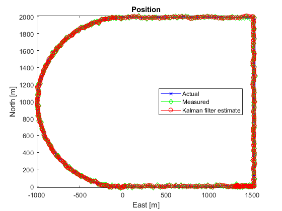
The error between the measured and actual position as well as the error between the Kalman filter estimate and actual position is:

% East position measurement error [m]
n_xe = y(:,1)-x(:,1);
% North position measurement error [m]
n_xn = y(:,2)-x(:,2);
% Kalman filter east position error [m]
e_xe = xhat(:,1)-x(:,1);
% Kalman filter north position error [m]
e_xn = xhat(:,2)-x(:,2);

figure;
% East Position Errors
subplot(2,1,1);
plot(t,n_xe,'g',t,e_xe,'r');
ylabel('Position Error - East [m]');
xlabel('Time [s]');
legend(sprintf('Meas: %.3f',norm(n_xe,1)/numel(n_xe)),...
    sprintf('Kalman f.: %.3f',norm(e_xe,1)/numel(e_xe)));
axis tight;
% North Position Errors
subplot(2,1,2);
plot(t,y(:,2)-x(:,2),'g',t,xhat(:,2)-x(:,2),'r');
ylabel('Position Error - North [m]');
xlabel('Time [s]');
legend(sprintf('Meas: %.3f',norm(n_xn,1)/numel(n_xn)),...
    sprintf('Kalman f: %.3f',norm(e_xn,1)/numel(e_xn)));
axis tight;

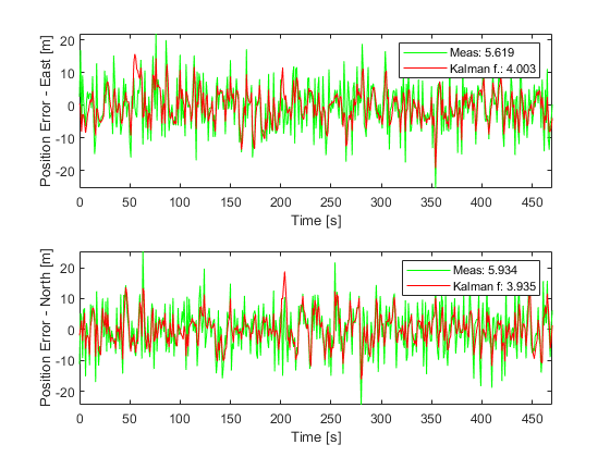
The plot legends show the position measurement and estimation error ( $||x_e-\hat{x}_e||_1$ and $||x_n-\hat{x}_n||_1$ ) normalized by the number of data points. The Kalman filter estimates have about 25% percent less error than the raw measurements.

The actual velocity in the east direction and its Kalman filter estimate is shown below in the top plot. The bottom plot shows the estimation error.

e_ve = xhat(:,3)-x(:,3); % [m/s] Kalman filter east velocity error
e_vn = xhat(:,4)-x(:,4); % [m/s] Kalman filter north velocity error
figure;
% Velocity in east direction and its estimate
subplot(2,1,1);
plot(t,x(:,3),'b',t,xhat(:,3),'r');
ylabel('Velocity - East [m/s]');
xlabel('Time [s]');
legend('Actual','Kalman filter','Location','Best');
axis tight;
subplot(2,1,2);
% Estimation error
plot(t,e_ve,'r');
ylabel('Velocity Error - East [m/s]');
xlabel('Time [s]');
legend(sprintf('Kalman filter: %.3f',norm(e_ve,1)/numel(e_ve)));
axis tight;

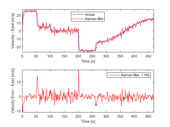
The legend on the error plot shows the east velocity estimation error $||\dot{x}_e-\hat{\dot{x}}_e||_1$ normalized by the number of data points.

The Kalman filter velocity estimates track the actual velocity trends correctly. The noise levels decrease when the vehicle is traveling at high velocities. This is in line with the design of the Q matrix. The large two spikes are at t=50s and t=200s. These are the times when the car goes through sudden deceleration and a sharp turn, respectively. The velocity changes at those instants are much larger than the predictions from the Kalman filter, which is based on its Q matrix input. After a few time-steps, the filter estimates catch up with the actual velocity.

Summary

You estimated the position and velocity of a vehicle using the Kalman filter block in Simulink. The process noise dynamics of the model were time-varying. You validated the filter performance by simulating various vehicle maneuvers and randomly generated measurement noise. The Kalman filter improved the position measurements and provided velocity estimates for the vehicle.

bdclose('ctrlKalmanNavigationExample');