Surface Fitting to Biopharmaceutical Data
Curve Fitting Toolbox™ software provides some example data for an anesthesia drug interaction study. You can use the Curve Fitter app to fit response surfaces to this data to analyze drug interaction effects. Response surface models provide a good method for understanding the pharmacodynamic interaction behavior of drug combinations. This data is based on the results in [1].
Anesthesia is typically at least a two-drug process, consisting of an opioid and a sedative hypnotic. This example uses Propofol and Reminfentanil as drug class prototypes. Their interaction is measured by four different measures of the analgesic and sedative response to the drug combination. Algometry, Tetany, Sedation, and Laryingoscopy comprise the four measures of surrogate drug effects at various concentration combinations of Propofol and Reminfentanil.
To interactively create response surfaces for this drug combination:
Use the Files panel to locate and view the folder
matlab\toolbox\curvefit\curvefit.Right-click the file
OpioidHypnoticSynergy.txt, and select Import Data. The Import Tool appears.On the Import tab, in the Delimiters section, leave the default Column delimiters value as
Tab.Review the six variables selected for import:
Propofol,Reminfentanil,Algometry,Tetany,Sedation, andLaryingoscopy.In the Import section, click Import Selection and select Import Data to import the dose-response data into the MATLAB® workspace. Close the Import Tool.
Alternatively, you can import the data programmatically. Enter the following code to read the dose-response data from the file into the MATLAB workspace.
data = importdata("OpioidHypnoticSynergy.txt");
OpioidHypnoticSynergy = array2table(data.data, ...
    "VariableNames",data.textdata);
To create response surfaces, you must select two drugs as x and y inputs, and one of the four effects as the z output. After you load the variables into your workspace, you open the Curve Fitter app and then select variables interactively. Alternatively, you can specify the initial fit variables when using the
curveFitterfunction.For this example, open the Curve Fitter app.
curveFitter
In the Curve Fitter app, on the Curve Fitter tab, in the Data section, click Select Data. In the Select Fitting Data dialog box, first select the
OpioidHypnoticSynergytable from the X data, Y data, and Z data drop-down lists. Then select thePropofol,Remifentanil, andAlgometryvariables from the new drop-down lists.
The app creates a new response surface for the
Algometrydata. The default fit is an interpolating surface that passes through the data points.
Create a copy of the current surface fit by either:
Selecting the Duplicate button in the File section of the Curve Fitter tab.
Right-clicking a fit in the Table Of Fits pane, and selecting Duplicate "untitled fit 1".
Define your own equation to fit the data. On the Curve Fitter tab, in the Fit Type section, click the arrow to open the gallery. In the gallery, click Custom Equation in the Custom group.
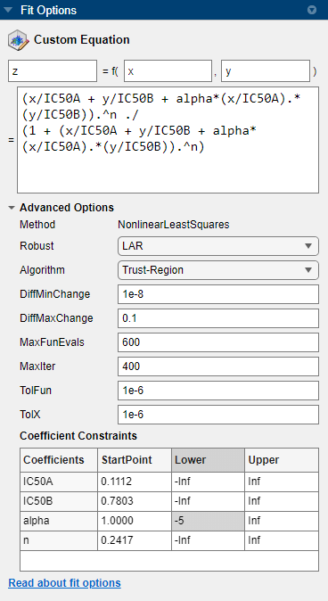
In the Fit Options pane, select and delete the example custom equation text in the edit box.
You can use the custom equation edit box to enter MATLAB code to define your model. The equation that defines the model must depend on the data variables
xandyand a list of fixed parameters, estimable parameters, or both.The model from the paper is:
where CA and CB are the drug concentrations, and IC50A, IC50B, alpha, and n are the coefficients to be estimated.
You can define this in MATLAB code as:
Effect = Emax*(CA/IC50A + CB/IC50B + ...
    alpha*(CA/IC50A).*(CB/IC50B)).^n ./ ...
    (1 + (CA/IC50A + CB/IC50B + ...
    alpha*(CA/IC50A ).*(CB/IC50B)).^n);
Telling the app which variables to fit and which parameters to estimate requires rewriting the variable names
CAandCBasx, andy. You must includexandywhen you enter a custom equation in the edit box. AssumeEmax = 1because the effect output is normalized.Enter the following text in the custom equation edit box.
(x/IC50A + y/IC50B + alpha*(x/IC50A).*(y/IC50B)).^n ./
(1 + (x/IC50A + y/IC50B + alpha*(x/IC50A).*(y/IC50B)).^n)
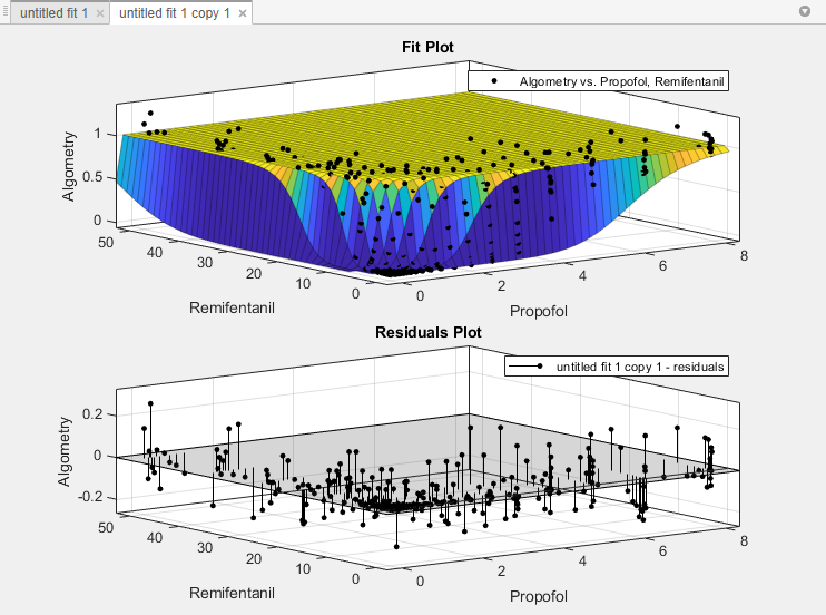
The Curve Fitter app fits a surface to the data using the custom equation model.

In the Fit Options pane, change some of the fit options. Click Advanced Options to expand the section.
Set the Robust value to
LAR.In the Coefficient Constraints table, for the alpha coefficient, set the StartPoint value to
1and the Lower bound to–5.
The app updates the fit with your new options.
Review the Results pane. View any of these results:
The model equation
The values of the estimated coefficients
The goodness-of-fit statistics
Display the residuals plot to check the distribution of points relative to the surface. On the Curve Fitter tab, in the Visualization section, click Residuals Plot.

Generate code for the currently selected fit and its open plots in your Curve Fitter app session. On the Curve Fitter tab, in the Export section, click Export and select Generate Code.
The Curve Fitter app generates code from your session and displays the file in the MATLAB Editor. The file includes the fit selected in your current session and its open plots.
Save the file with the default name,
createFit.m.You can recreate your fit and its plots by calling the file from the command line with your original data or new data as input arguments.
In this case, because your original data still appears in the workspace, you can run the function with the original data variables.
[fitresult,gof] = createFit(OpioidHypnoticSynergy.Propofol, ...
    OpioidHypnoticSynergy.Remifentanil, ...
    OpioidHypnoticSynergy.Algometry)
The function creates a figure window for the fit you selected in your session. The custom fit figure shows both the surface and residuals plots that you created interactively in the Curve Fitter app.
Create a new fit to the
Tetanyresponse instead ofAlgometry.[fitresult,gof] = createFit(OpioidHypnoticSynergy.Propofol, ... OpioidHypnoticSynergy.Remifentanil, ... OpioidHypnoticSynergy.Tetany)
You need to edit the file if you want the new response label on the plots. You can use the generated code as a starting point to change the surface fits and plots to meet your needs. For a list of methods you can use, see
sfit.
To see how to programmatically fit surfaces to the same example problem, see Surface Fitting with Custom Equations to Biopharmaceutical Data.
References
[1] Kern, Steven E., Guoming Xie, Julia L. White, and Talmage D. Egan. “A Response Surface Analysis of Propofol–Remifentanil Pharmacodynamic Interaction in Volunteers.” Anesthesiology 100, no. 6 (June 1, 2004): 1373–81. https://doi.org/10.1097/00000542-200406000-00007.