对数据进行指数模型拟合
此示例说明如何使用信赖域和莱文贝格-马夸特非线性最小二乘算法对数据进行指数模型拟合。
加载 census 数据集。
load census变量 pop 和 cdate 分别包含人口规模和人口普查年份的数据。
显示数据的散点图。
scatter(cdate,pop)
xlabel("Year")
ylabel("Population")

绘图显示人口以类似指数函数的形式逐年增长。
使用默认信赖域拟合算法对人口数据进行双项指数模型拟合。返回拟合结果和拟合优度统计量。
[exp_tr,gof_tr] = fit(cdate,pop,"exp2")exp_tr =
General model Exp2:
exp_tr(x) = a*exp(b*x) + c*exp(d*x)
Coefficients (with 95% confidence bounds):
a = 7.169e-17
b = 0.02155
c = 0
d = 0.02155
gof_tr = struct with fields:
           sse: 1.2412e+04
       rsquare: 0.8995
           dfe: 17
    adjrsquare: 0.8818
          rmse: 27.0209
exp_tr 包含拟合的结果,包括用信赖域拟合算法计算的系数。存储在 gof_tr 中的拟合优度统计量包括均方根误差 (RMSE) 值 27.0209。
绘制 exp_tr 中模型的图以及数据散点图。
plot(exp_tr,cdate,pop)
legend(["data","predicted value"])
xlabel("Year")
ylabel("Population")

绘图显示 exp_tr 中的模型与人口普查数据并未紧密吻合。
通过使用莱文贝格-马夸特拟合算法计算系数来改进拟合。
[exp_lm,gof_lm] = fit(cdate,pop,"exp2",Algorithm="Levenberg-Marquardt")
exp_lm =
     General model Exp2:
     exp_lm(x) = a*exp(b*x) + c*exp(d*x)
     Coefficients (with 95% confidence bounds):
       a =   4.282e-17  (-1.125e-11, 1.126e-11)
       b =     0.02477  (-5.67, 5.719)
       c =  -3.933e-17  (-1.126e-11, 1.126e-11)
       d =     0.02481  (-5.696, 5.745)
gof_lm = struct with fields:
           sse: 475.9498
       rsquare: 0.9961
           dfe: 17
    adjrsquare: 0.9955
          rmse: 5.2912
exp_lm 包含拟合的结果,包括用莱文贝格-马夸特拟合算法计算的系数。存储在 gof_lm 中的拟合优度统计量包括 RMSE 值 5.2912,它小于 exp_tr 的 RMSE。RMSE 的相对大小表明,存储在 exp_lm 中的模型比存储在 exp_tr 中的模型对数据的拟合更准确。
绘制 exp_lm 中模型的图以及数据散点图。
plot(exp_lm,cdate,pop)
legend(["data","predicted value"])
xlabel("Year")
ylabel("Population")
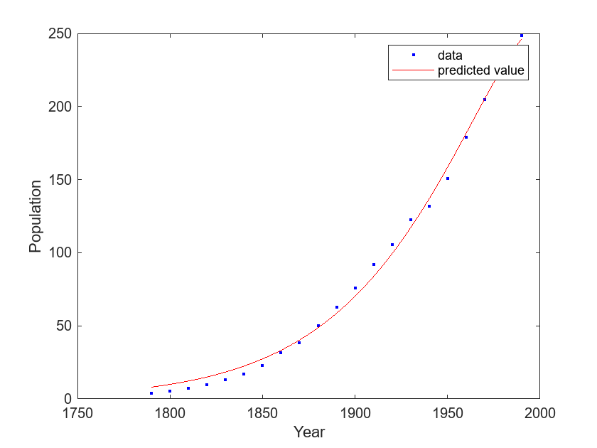
绘图显示 exp_lm 中的模型比 exp_tr 中的模型与人口普查数据的吻合程度更高。